Why Stuff Can Orbit, Part 9: How The Spring In The Cosmos Behaves

Why Stuff Can Orbit, featuring a dazed-looking coati (it's a raccoon-like creature from Latin America) and a starry background. — Art courtesy of Thomas K Dye, creator of the web comic **Newshounds**. He has a Patron for those able to support his work.

Previously:

And the supplemental reading:

First, I thank Thomas K Dye for the banner art I have for this feature! Thomas is the creator of the longrunning web comic Newshounds. He’s hoping soon to finish up special editions of some of the strip’s stories and to publish a definitive edition of the comic’s history. He’s also got a Patreon account to support his art habit. Please give his creations some of your time and attention.

Now back to central forces. I’ve run out of obvious fun stuff to say about a mass that’s in a circular orbit around the center of the universe. Before you question my sense of fun, remember that I own multiple pop histories about the containerized cargo industry and last month I read another one that’s changed my mind about some things. These sorts of problems cover a lot of stuff. They cover planets orbiting a sun and blocks of wood connected to springs. That’s about all we do in high school physics anyway. Well, there’s spheres colliding, but there’s no making a central force problem out of those. You can also make some things that look like bad quantum mechanics models out of that. The mathematics is interesting even if the results don’t match anything in the real world.

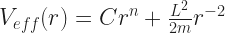
But I’m sticking with central forces that look like powers. These have potential energy functions with rules that look like V(r) = C rⁿ. So far, ‘n’ can be any real number. It turns out ‘n’ has to be larger than -2 for a circular orbit to be stable, but that’s all right. There are lots of numbers larger than -2. ‘n’ carries the connotation of being an integer, a whole (positive or negative) number. But if we want to let it be any old real number like 0.1 or π or 18 and three-sevenths that’s fine. We make a note of that fact and remember it right up to the point we stop pretending to care about non-integer powers. I estimate that’s like two entries off.

We get a circular orbit by setting the thing that orbits in … a circle. This sounded smarter before I wrote it out like that. Well. We set it moving perpendicular to the “radial direction”, which is the line going from wherever it is straight to the center of the universe. This perpendicular motion means there’s a non-zero angular momentum, which we write as ‘L’ for some reason. For each angular momentum there’s a particular radius that allows for a circular orbit. Which radius? It’s whatever one is a minimum for the effective potential energy:

$V_{eff}(r) = Cr^n + \frac{L^2}{2m}r^{-2}$

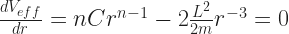
This we can find by taking the first derivative of ‘V_eff‘ with respect to ‘r’ and finding where that first derivative is zero. This is standard mathematics stuff, quite routine. We can do with any function whether it represents something physics or not. So:

$\frac{dV_{eff}}{dr} = nCr^{n-1} - 2\frac{L^2}{2m}r^{-3} = 0$

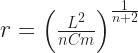
And after some work, this gets us to the circular orbit’s radius:

$r = \left(\frac{L^2}{nCm}\right)^{\frac{1}{n + 2}}$

What I’d like to talk about is if we’re not quite at that radius. If we set the planet (or whatever) a little bit farther from the center of the universe. Or a little closer. Same angular momentum though, so the equilibrium, the circular orbit, should be in the same spot. It happens there isn’t a planet there.

This enters us into the world of perturbations, which is where most of the big money in mathematical physics is. A perturbation is a little nudge away from an equilibrium. What happens in response to the little nudge is interesting stuff. And here we already know, qualitatively, what’s going to happen: the planet is going to rock around the equilibrium. This is because the circular orbit is a stable equilibrium. I’d described that qualitatively last time. So now I want to talk quantitatively about how the perturbation changes given time.

Before I get there I need to introduce another bit of notation. It is so convenient to be able to talk about the radius of the circular orbit that would be the equilibrium. I’d called that ‘r’ up above. But I also need to be able to talk about how far the perturbed planet is from the center of the universe. That’s also really hard not to call ‘r’. Something has to give. Since the radius of the circular orbit is not going to change I’m going to give that a new name. I’ll call it ‘a’. There’s several reasons for this. One is that ‘a’ is commonly used for describing the size of ellipses, which turn up in actual real-world planetary orbits. That’s something we know because this is like the thirteenth part of an essay series about the mathematics of orbits. You aren’t reading this if you haven’t picked up a couple things about orbits on your own. Also we’ve used ‘a’ before, in these sorts of approximations. It was handy in the last supplemental as the point of expansion’s name. So let me make that unmistakable:

$a \equiv r = \left(\frac{L^2}{nCm}\right)^{\frac{1}{n + 2}}$

The $\equiv$ there means “defined to be equal to”. You might ask how this is different from “equals”. It seems like more emphasis to me. Also, there are other names for the circular orbit’s radius that I could have used. ‘r_e‘ would be good enough, as the subscript would suggest “radius of equilibrium”. Or ‘r₀‘ would be another popular choice, the 0 suggesting that this is something of key, central importance and also looking kind of like a circle. (That’s probably coincidence.) I like the ‘a’ better there because I know how easy it is to drop a subscript. If you’re working on a problem for yourself that’s easy to fix, with enough cursing and redoing your notes. On a board in front of class it’s even easier to fix since someone will ask about the lost subscript within three lines. In a post like this? It would be a mess.

So now I’m going to look at possible values of the radius ‘r’ that are close to ‘a’. How close? Close enough that ‘V_eff‘, the effective potential energy, looks like a parabola. If it doesn’t look much like a parabola then I look at values of ‘r’ that are even closer to ‘a’. (Do you see how the game is played? If you don’t, look closer. Yes, this is actually valid.) If ‘r’ is that close to ‘a’, then we can get away with this polynomial expansion:

$V_{eff}(r) \approx V_{eff}(a) + m\cdot(r - a) + \frac{1}{2} m_2 (r - a)^2$

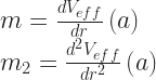
where

$m = \frac{dV_{eff}}{dr}\left(a\right) \\ m_2 = \frac{d^2V_{eff}}{dr^2}\left(a\right)$

The “approximate” there is because this is an approximation. $V_{eff}(r)$ is in truth equal to the thing on the right-hand-side there plus something that isn’t (usually) zero, but that is small.

I am sorry beyond my ability to describe that I didn’t make that ‘m’ and ‘m₂‘ consistent last week. That’s all right. One of these is going to disappear right away.

Now, what $V_{eff}(a)$ is? Well, that’s whatever you get from putting in ‘a’ wherever you start out seeing ‘r’ in the expression for $V_{eff}(r)$ . I’m not going to bother with that. Call it math, fine, but that’s just a search-and-replace on the character ‘r’. Also, where I’m going next, it’s going to disappear, never to be seen again, so who cares? What’s important is that this is a constant number. If ‘r’ changes, the value of $V_{eff}(a)$ does not, because ‘r’ doesn’t appear anywhere in $V_{eff}(a)$ .

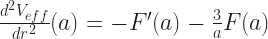
How about ‘m’? That’s the value of the first derivative of ‘V_eff‘ with respect to ‘r’, evaluated when ‘r’ is equal to ‘a’. That might be something. It’s not, because of what ‘a’ is. It’s the value of ‘r’ which would make $\frac{dV_{eff}}{dr}(r)$ equal to zero. That’s why ‘a’ has that value instead of some other, any other.

So we’ll have a constant part ‘V_eff(a)’, plus a zero part, plus a part that’s a parabola. This is normal, by the way, when we do expansions around an equilibrium. At least it’s common. Good to see it. To find ‘m₂‘ we have to take the second derivative of ‘V_eff(r)’ and then evaluate it when ‘r’ is equal to ‘a’ and ugh but here it is.

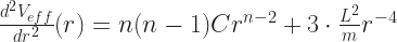
$\frac{d^2V_{eff}}{dr^2}(r) = n (n - 1) C r^{n - 2} + 3\cdot\frac{L^2}{m}r^{-4}$

And at the point of approximation, where ‘r’ is equal to ‘a’, it’ll be:

$m_2 = \frac{d^2V_{eff}}{dr^2}(a) = n (n - 1) C a^{n - 2} + 3\cdot\frac{L^2}{m}a^{-4}$

We know exactly what ‘a’ is so we could write that out in a nice big expression. You don’t want to. I don’t want to. It’s a bit of a mess. I mean, it’s not hard, but it has a lot of symbols in it and oh all right. Here. Look fast because I’m going to get rid of that as soon as I can.

$m_2 = \frac{d^2V_{eff}}{dr^2}(a) = n (n - 1) C \left(\frac{L^2}{n C m}\right)^{n - 2} + 3\cdot\frac{L^2}{m}\left(\frac{L^2}{n C m}\right)^{-4}$

For the values of ‘n’ that we actually care about because they turn up in real actual physics problems this expression simplifies some. Enough, anyway. If we pretend we know nothing about ‘n’ besides that it is a number bigger than -2 then … ugh. We don’t have a lot that can clean it up.

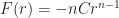
Here’s how. I’m going to define an auxiliary little function. Its role is to contain our symbolic sprawl. It has a legitimate role too, though. At least it represents something that it makes sense to give a name. It will be a new function, named ‘F’ and that depends on the radius ‘r’:

$F(r) \equiv -\frac{dV}{dr}$

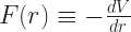
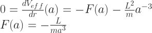
Notice that’s the derivative of the original ‘V’, not the angular-momentum-equipped ‘V_eff‘. This is the secret of its power. It doesn’t do anything to make $V_{eff}(r)$ easier to work with. It starts being good when we take its derivatives, though:

$\frac{dV_{eff}}{dr} = -F(r) - \frac{L^2}{m}r^{-3}$

That already looks nicer, doesn’t it? It’s going to be really slick when you think about what ‘F(a)’ is. Remember that ‘a’ is the value for ‘r’ which makes the derivative of ‘V_eff‘ equal to zero. So … I may not know much, but I know this:

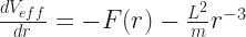
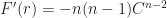
$0 = \frac{dV_{eff}}{dr}(a) = -F(a) - \frac{L^2}{m}a^{-3} \\ F(a) = -\frac{L}{ma^3}$

I’m not going to say what value F(r) has for other values of ‘r’ because I don’t care. But now look at what it does for the second derivative of ‘V_eff‘:

$\frac{d^2 V_{eff}}{dr^2}(r) = -F'(r) + 3\frac{L^2}{mr^4}$

Here the ‘F'(r)’ is a shorthand way of writing ‘the derivative of F with respect to r’. You can do when there’s only the one free variable to consider. And now something magic that happens when we look at the second derivative of ‘V_eff‘ when ‘r’ is equal to ‘a’ …

$\frac{d^2 V_{eff}}{dr^2}(a) = -F'(a) - \frac{3}{a} F(a)$

We get away with this because we happen to know that ‘F(a)’ is equal to $-\frac{L}{ma^3}$ and doesn’t that work out great? We’ve turned a symbolic mess into a … less symbolic mess.

Now why do I say it’s legitimate to introduce ‘F(r)’ here? It’s because minus the derivative of the potential energy with respect to the position of something can be something of actual physical interest. It’s the amount of force exerted on the particle by that potential energy at that point. The amount of force on a thing is something that we could imagine being interested in. Indeed, we’d have used that except potential energy is usually so much easier to work with. I’ve avoided it up to this point because it wasn’t giving me anything I needed. Here, I embrace it because it will save me from some awful lines of symbols.

Because with this expression in place I can write the approximation to the potential energy of:

$V_{eff}(r) \approx V_{eff}(a) + \frac{1}{2} \left( -F'(a) - \frac{3}{a}F(a) \right) (r - a)^2$

So if ‘r’ is close to ‘a’, then the polynomial on the right is a good enough approximation to the effective potential energy. And that potential energy has the shape of a spring’s potential energy. We can use what we know about springs to describe its motion. Particularly, we’ll have this be true:

$\frac{dp}{dt} = -\frac{dv_{eff}}{dr}(r) = -\left( F'(a) + \frac{3}{a} F(a)\right) r$

Here, ‘p’ is the (linear) momentum of whatever’s orbiting, which we can treat as equal to ‘mr’, the mass of the orbiting thing times how far it is from the center. You may sense in me some reluctance about doing this, what with that ‘we can treat as equal to’ talk. There’s reasons for this and I’d have to get deep into geometry to explain why. I can get away with specifically this use because the problem allows it. If you’re trying to do your own original physics problem inspired by this thread, and it’s not orbits like this, be warned. This is a spot that could open up to a gigantic danger pit, lined at the bottom with sharp spikes and angry poison-clawed mathematical tigers and I bet it’s raining down there too.

So we can rewrite all this as

$m\frac{d^2r}{dt^2} = -\frac{dv_{eff}}{dr}(r) = -\left( F'(a) + \frac{3}{a} F(a)\right) r$

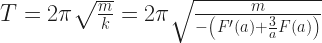
And when we learned everything interesting there was to know about springs we learned what the solutions to this look like. Oh, in that essay the variable that changed over time was called ‘x’ and here it’s called ‘r’, but that’s not an actual difference. ‘r’ will be some sinusoidal curve:

$r(t) = A cos\left(\sqrt{\frac{k}{m}} t\right) + B sin\left(\sqrt{\frac{k}{m}} t\right)$

where, here, ‘k’ is equal to that whole mass of constants on the right-hand side:

$k = -\left( F'(a) + \frac{3}{a} F(a)\right)$

I don’t know what ‘A’ and ‘B’ are. It’ll depend on just what the perturbation is like, how far the planet is from the circular orbit. But I can tell you what the behavior is like. The planet will wobble back and forth around the circular orbit, sometimes closer to the center, sometimes farther away. It’ll spend as much time closer to the center than the circular orbit as it does farther away. And the period of that oscillation will be

$T = 2\pi\sqrt{\frac{m}{k}} = 2\pi\sqrt{\frac{m}{-\left(F'(a) + \frac{3}{a}F(a)\right)}}$

This tells us something about what the orbit of a thing not in a circular orbit will be like. Yes, I see you in the back there, quivering with excitement about how we’ve got to elliptical orbits. You’re moving too fast. We haven’t got that. There will be elliptical orbits, yes, but only for a very particular power ‘n’ for the potential energy. Not for most of them. We’ll see.

It might strike you there’s something in that square root. We need to take the square root of a positive number, so maybe this will tell us something about what kinds of powers we’re allowed. It’s a good thought. It turns out not to tell us anything useful, though. Suppose we started with $V(r) = Cr^n$ . Then $F(r) = -nCr^{n - 1}$ , and $F'(r) = -n(n - 1)C^{n - 2}$ . Sad to say, this leads us to a journey which reveals that we need ‘n’ to be larger than -2 or else we don’t get oscillations around a circular orbit. We already knew that, though. We already found we needed it to have a stable equilibrium before. We can see there not being a period for these oscillations around the circular orbit as another expression of the circular orbit not being stable. Sad to say, we haven’t got something new out of this.

We will get to new stuff, though. Maybe even ellipses.

Author: Joseph Nebus

I was born 198 years to the day after Johnny Appleseed. The differences between us do not end there. He/him. View all posts by Joseph Nebus

Why Stuff Can Orbit, Part 9: How The Spring In The Cosmos Behaves

Author: Joseph Nebus

5 thoughts on “Why Stuff Can Orbit, Part 9: How The Spring In The Cosmos Behaves”

Please Write Something Good Cancel reply

Kindly share this:

Related

Author: Joseph Nebus

5 thoughts on “Why Stuff Can Orbit, Part 9: How The Spring In The Cosmos Behaves”

Please Write Something Good Cancel reply