Previously:
And some supplemental reading:
So now we can work out orbits. At least orbits for a central force problem. Those are ones where a particle — it’s easy to think of it as a planet — is pulled towards the center of the universe. How strong that pull is depends on some constants. But it only changes as the distance the planet is from the center changes.
What we’d like to know is whether there are circular orbits. By “we” I mean “mathematical physicists”. And I’m including you in that “we”. If you’re reading this far you’re at least interested in knowing how mathematical physicists think about stuff like this.
It’s easiest describing when these circular orbits exist if we start with the potential energy. That’s a function named ‘V’. We write it as ‘V(r)’ to show it’s an energy that changes as ‘r’ changes. By ‘r’ we mean the distance from the center of the universe. We’d use ‘d’ for that except we’re so used to thinking of distance from the center as ‘radius’. So ‘r’ seems more compelling. Sorry.
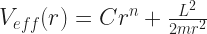
Besides the potential energy we need to know the angular momentum of the planet (or whatever it is) moving around the center. The amount of angular momentum is a number we call ‘L’. It might be positive, it might be negative. Also we need the planet’s mass, which we call ‘m’. The angular momentum and mass let us write a function called the effective potential energy, ‘Veff(r)’.
And we’ll need to take derivatives of ‘Veff(r)’. Fortunately that “How Differential Calculus Works” essay explains all the symbol-manipulation we need to get started. That part is calculus, but the easy part. We can just follow the rules already there. So here’s what we do:
- The planet (or whatever) can have a circular orbit around the center at any radius which makes the equation
 true.
true.
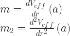
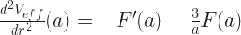
- The circular orbit will be stable if the radius of its orbit makes the second derivative of the effective potential,
 , some number greater than zero.
We’re interested in stable orbits because usually unstable orbits are boring. They might exist but any little perturbation breaks them down. The mathematician, ordinarily, sees this as a useless solution except in how it describes different kinds of orbits. The physicist might point out that sometimes it can take a long time, possibly millions of years, before the perturbation becomes big enough to stand out. Indeed, it’s an open question whether our solar system is stable. While it seems to have gone millions of years without any planet changing its orbit very much we haven’t got the evidence to say it’s impossible that, say, Saturn will be kicked out of the solar system anytime soon. Or worse, that Earth might be. “Soon” here means geologically soon, like, in the next million years.
(If it takes so long for the instability to matter then the mathematician might allow that as “metastable”. There are a lot of interesting metastable systems. But right now, I don’t care.)
I realize now I didn’t explain the notation for the second derivative before. It looks funny because that’s just the best we can work out. In that fraction the ‘d’ isn’t a number so we can’t cancel it out. And the superscript ‘2’ doesn’t mean squaring, at least not the way we square numbers. There’s a functional analysis essay in there somewhere. Again I’m sorry about this but there’s a lot of things mathematicians want to write out and sometimes we can’t find a way that avoids all confusion. Roll with it.
So that explains the whole thing clearly and easily and now nobody could be confused and yeah I know. If my Classical Mechanics professor left it at that we’d have open rebellion. Let’s do an example.
There are two and a half good examples. That is, they’re central force problems with answers we know. One is gravitation: we have a planet orbiting a star that’s at the origin. Another is springs: we have a mass that’s connected by a spring to the origin. And the half is electric: put a positive electric charge at the center and have a negative charge orbit that. The electric case is only half a problem because it’s the same as the gravitation problem except for what the constants involved are. Electric charges attract each other crazy way stronger than gravitational masses do. But that doesn’t change the work we do.
This is a lie. Electric charges accelerating, and just orbiting counts as accelerating, cause electromagnetic effects to happen. They give off light. That’s important, but it’s also complicated. I’m not going to deal with that.
I’m going to do the gravitation problem. After all, we know the answer! By Kepler’s something law, something something radius cubed something G M … something … squared … After all, we can look up the answer!
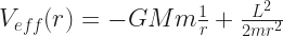
The potential energy for a planet orbiting a sun looks like this:

Here ‘G’ is a constant, called the Gravitational Constant. It’s how strong gravity in the universe is. It’s not very strong. ‘M’ is the mass of the sun. ‘m’ is the mass of the planet. To make sense ‘M’ should be a lot bigger than ‘m’. ‘r’ is how far the planet is from the sun. And yes, that’s one-over-r, not one-over-r-squared. This is the potential energy of the planet being at a given distance from the sun. One-over-r-squared gives us how strong the force attracting the planet towards the sun is. Different thing. Related thing, but different thing. Just listing all these quantities one after the other means ‘multiply them together’, because mathematicians multiply things together a lot and get bored writing multiplication symbols all the time.
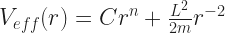
Now for the effective potential we need to toss in the angular momentum. That’s ‘L’. The effective potential energy will be:
I’m going to rewrite this in a way that means the same thing, but that makes it easier to take derivatives. At least easier to me. You’re on your own. But here’s what looks easier to me:

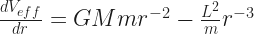
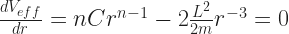
I like this because it makes every term here look like “some constant number times r to a power”. That’s easy to take the derivative of. Check back on that “How Differential Calculus Works” essay. The first derivative of this ‘Veff(r)’, taken with respect to ‘r’, looks like this:

We can tidy that up a little bit: -(-1) is another way of writing 1. The second term has two times something divided by 2. We don’t need to be that complicated. In fact, when I worked out my notes I went directly to this simpler form, because I wasn’t going to be thrown by that. I imagine I’ve got people reading along here who are watching these equations warily, if at all. They’re ready to bolt at the first sign of something terrible-looking. There’s nothing terrible-looking coming up. All we’re doing from this point on is really arithmetic. It’s multiplying or adding or otherwise moving around numbers to make the equation prettier. It happens we only know those numbers by cryptic names like ‘G’ or ‘L’ or ‘M’. You can go ahead and pretend they’re ‘4’ or ‘5’ or ‘7’ if you like. You know how to do the steps coming up.
So! We allegedly can have a circular orbit when this first derivative is equal to zero. What values of ‘r’ make true this equation?

Not so helpful there. What we want is to have something like ‘r = (mathematics stuff here)’. We have to do some high school algebra moving-stuff-around to get that. So one thing we can do to get closer is add the quantity  to both sides of this equation. This gets us:
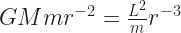
Things are getting better. Now multiply both sides by the same number. Which number? r3. That’s because ‘r-3‘ times ‘r3‘ is going to equal 1, while ‘r-2‘ times ‘r3‘ will equal ‘r1‘, which normal people call ‘r’. I kid; normal people don’t think of such a thing at all, much less call it anything. But if they did, they’d call it ‘r’. We’ve got:

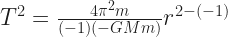
And now we’re getting there! Divide both sides by whatever number ‘G M’ is, as long as it isn’t zero. And then we have our circular orbit! It’s at the radius

Very good. I’d even say pretty. It’s got all those capital letters and one little lowercase. Something squared in the numerator and the denominator. Aesthetically pleasant. Stinks a little that it doesn’t look like anything we remember from Kepler’s Laws once we’ve looked them up. We can fix that, though.
The key is the angular momentum ‘L’ there. I haven’t said anything about how that number relates to anything. It’s just been some constant of the universe. In a sense that’s fair enough. Angular momentum is conserved, exactly the same way energy is conserved, or the way linear momentum is conserved. Why not just let it be whatever number it happens to be?
(A note for people who skipped earlier essays: Angular momentum is not a number. It’s really a three-dimensional vector. But in a central force problem with just one planet moving around we aren’t doing any harm by pretending it’s just a number. We set it up so that the angular momentum is pointing directly out of, or directly into, the sheet of paper we pretend the planet’s orbiting in. Since we know the direction before we even start work, all we have to care about is the size. That’s the number I’m talking about.)
The angular momentum of a thing is its moment of inertia times its angular velocity. I’m glad to have cleared that up for you. The moment of inertia of a thing describes how easy it is to start it spinning, or stop it spinning, or change its spin. It’s a lot like inertia. What it is depends on the mass of the thing spinning, and how that mass is distributed, and what it’s spinning around. It’s the first part of physics that makes the student really have to know volume integrals.
We don’t have to know volume integrals. A single point mass spinning at a constant speed at a constant distance from the origin is the easy angular momentum to figure out. A mass ‘m’ at a fixed distance ‘r’ from the center of rotation moving at constant speed ‘v’ has an angular momentum of ‘m’ times ‘r’ times ‘v’.
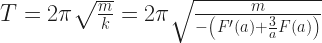
So great; we’ve turned ‘L’ which we didn’t know into ‘m r v’, where we know ‘m’ and ‘r’ but don’t know ‘v’. We’re making progress, I promise. The planet’s tracing out a circle in some amount of time. It’s a circle with radius ‘r’. So it traces out a circle with perimeter ‘2 π r’. And it takes some amount of time to do that. Call that time ‘T’. So its speed will be the distance travelled divided by the time it takes to travel. That’s  . Again we’ve changed one unknown number ‘L’ for another unknown number ‘T’. But at least ‘T’ is an easy familiar thing: it’s how long the orbit takes.
Let me show you how this helps. Start off with what ‘L’ is:

Now let’s put that into the equation I got eight paragraphs ago:
Remember that one? Now put what I just said ‘L’ was, in where ‘L’ shows up in that equation.

I agree, this looks like a mess and possibly a disaster. It’s not so bad. Do some cleaning up on that numerator.

That’s looking a lot better, isn’t it? We even have something we can divide out: the mass of the planet is just about to disappear. This sounds bizarre, but remember Kepler’s laws: the mass of the planet never figures into things. We may be on the right path yet.

OK. Now I’m going to multiply both sides by ‘T2‘ because that’ll get that out of the denominator. And I’ll divide both sides by ‘r’ so that I only have the radius of the circular orbit on one side of the equation. Here’s what we’ve got now:

And hey! That looks really familiar. A circular orbit’s radius cubed is some multiple of the square of the orbit’s time. Yes. This looks right. At least it looks reasonable. Someone else can check if it’s right. I like the look of it.
So this is the process you’d use to start understanding orbits for your own arbitrary potential energy. You can find the equivalent of Kepler’s Third Law, the one connecting orbit times and orbit radiuses. And it isn’t really hard. You need to know enough calculus to differentiate one function, and then you need to be willing to do a pile of arithmetic on letters. It’s not actually hard. Next time I hope to talk about more and different … um …
I’d like to talk about the different … oh, dear. Yes. You’re going to ask about that, aren’t you?
Ugh. All right. I’ll do it.
How do we know this is a stable orbit? Well, it just is. If it weren’t the Earth wouldn’t have a Moon after all this. Heck, the Sun wouldn’t have an Earth. At least it wouldn’t have a Jupiter. If the solar system is unstable, Jupiter is probably the most stable part. But that isn’t convincing. I’ll do this right, though, and show what the second derivative tells us. It tells us this is too a stable orbit.
So. The thing we have to do is find the second derivative of the effective potential. This we do by taking the derivative of the first derivative. Then we have to evaluate this second derivative and see what value it has for the radius of our circular orbit. If that’s a positive number, then the orbit’s stable. If that’s a negative number, then the orbit’s not stable. This isn’t hard to do, but it isn’t going to look pretty.
First the pretty part, though. Here’s the first derivative of the effective potential:
OK. So the derivative of this with respect to ‘r’ isn’t hard to evaluate again. This is again a function with a bunch of terms that are all a constant times r to a power. That’s the easiest sort of thing to differentiate that isn’t just something that never changes.

Now the messy part. We need to work out what that line above is when our planet’s in our circular orbit. That circular orbit happens when  . So we have to substitute that mess in for ‘r’ wherever it appears in that above equation and you’re going to love this. Are you ready? It’s:

This will get a bit easier promptly. That’s because something raised to a negative power is the same as its reciprocal raised to the positive of that power. So that terrible, terrible expression is the same as this terrible, terrible expression:

Yes, yes, I know. Only thing to do is start hacking through all this because I promise it’s going to get better. Putting all those third- and fourth-powers into their parentheses turns this mess into:

Yes, my gut reaction when I see multiple things raised to the eighth power is to say I don’t want any part of this either. Hold on another line, though. Things are going to start cancelling out and getting shorter. Group all those things-to-powers together:
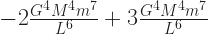
Oh. Well, now this is different. The second derivative of the effective potential, at this point, is the number

And I admit I don’t know what number that is. But here’s what I do know: ‘G’ is a positive number. ‘M’ is a positive number. ‘m’ is a positive number. ‘L’ might be positive or might be negative, but ‘L6‘ is a positive number either way. So this is a bunch of positive numbers multiplied and divided together.
So this second derivative what ever it is must be a positive number. And so this circular orbit is stable. Give the planet a little nudge and that’s all right. It’ll stay near its orbit. I’m sorry to put you through that but some people raised the, honestly, fair question.
So this is the process you’d use to start understanding orbits for your own arbitrary potential energy. You can find the equivalent of Kepler’s Third Law, the one connecting orbit times and orbit radiuses. And it isn’t really hard. You need to know enough calculus to differentiate one function, and then you need to be willing to do a pile of arithmetic on letters. It’s not actually hard. Next time I hope to talk about the other kinds of central forces that you might get. We only solved one problem here. We can solve way more than that.


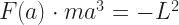
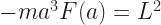
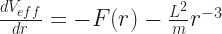
 . It’s convenient to have around. It makes equations like this one simpler, for one. And it’s weird to think of a central force problem where we never, ever see forces. The peculiar thing is we define ‘F’ for every distance the planet might be from the center of the universe. But all we care about is its value at the equilibrium, circular orbit distance of ‘a’. We also care about its first derivative, also evaluated at the distance of ‘a’, which is that
  talk early on in that denominator.


 at least as long as ‘ma2‘ is positive. It is.


 , not 90 degrees, thank you. A full circle is
  and not 360 degrees. We aren’t doing this to be difficult. There are good reasons to use radians. They make the mathematics simpler. What else could matter?
  as the symbol for this angle. It’s a popular choice.
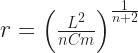
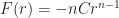
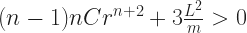
  for some number ‘C’ and some power, another number, ‘n’. Suppose your planet has the mass ‘m’. Then you’ll get a circular orbit when the planet’s a distance ‘a’ from the center, if
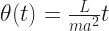
  . And it turns out we can also work out the angular velocity of this circular orbit. It’s all implicit in the amount of angular momentum that the planet has. This is part of why a mathematical physicist looks for concepts like angular momentum. They’re easy to work with, and they yield all sorts of interesting information, given the chance.
  , and we know
  , we have
  and from this:


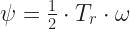
 is the angular velocity. The angular velocity is a vector that describes for us how fast the spinning is and what direction the axis around which the thing spins is. The moment of inertia describes how easy or hard it is to make the thing spin around each axis. It’s


 there means “defined to be equal to”. You might ask how this is different from “equals”. It seems like more emphasis to me. Also, there are other names for the circular orbit’s radius that I could have used. ‘re‘ would be good enough, as the subscript would suggest “radius of equilibrium”. Or ‘r0‘ would be another popular choice, the 0 suggesting that this is something of key, central importance and also looking kind of like a circle. (That’s probably coincidence.) I like the ‘a’ better there because I know how easy it is to drop a subscript. If you’re working on a problem for yourself that’s easy to fix, with enough cursing and redoing your notes. On a board in front of class it’s even easier to fix since someone will ask about the lost subscript within three lines. In a post like this? It would be a mess.
 is in truth equal to the thing on the right-hand-side there plus something that isn’t (usually) zero, but that is small.
  is? Well, that’s whatever you get from putting in ‘a’ wherever you start out seeing ‘r’ in the expression for
  equal to zero. That’s why ‘a’ has that value instead of some other, any other.
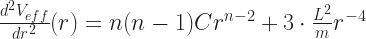


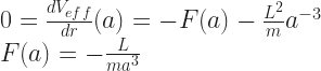

 and doesn’t that work out great? We’ve turned a symbolic mess into a … less symbolic mess.


 , and
, and 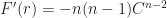 . Sad to say, this leads us to a journey which reveals that we need ‘n’ to be larger than -2 or else we don’t get oscillations around a circular orbit.
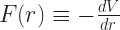
 — also known as
  if that looks better — is “the derivative of p with respect to t”. It means “how the value of the momentum changes as the time changes”. And that is equal to minus one times …
  — also written as
  — is some kind of derivative. The
  looks kind of like a cursive d, after all. It’s known as the partial derivative, because it means we look at how ‘U’ changes as ‘x’ and nothing else at all changes. With the normal, ‘d’ style full derivative, we have to track how all the variables change as the ‘t’ we’re interested in changes. In this particular problem the difference doesn’t matter. But there are problems where it does matter and that’s why I’m careful about the symbols.
 . The mass of your thing isn’t changing. If you’re going to let it change then we’re doing some screwy rocket problem and that’s a different article. So its easy to get the momentum out of that problem. We get instead the second derivative of the displacement with respect to time:

 with respect to ‘t’ is
  . The second derivative with respect to ‘t’ is
  . so here’s what we have:
 on the left side has to equal the
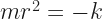


 . So that product has to be the initial velocity. That’s not much harder.


 to both sides of the equation; we’re used to doing that. At least in high school algebra we are.


 is the same number as
  . So we have this bit of distribution-law magic:

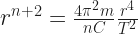
 . So we put that in where ‘rn+2‘ appeared in that above expression.

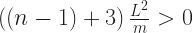
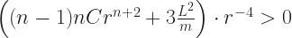
 has to be positive. The angular momentum ‘L’ might be positive or might be negative but its square is certainly positive. The mass ‘m’ has to be a positive number. So we’ll get a stable equilibrium whenever
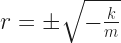
  is greater than 0. That is, whenever
  . Done.
  you wouldn’t have any orbits at all, never mind stable orbits. But 3 is certainly greater than -2. So what’s gone wrong here?
 . ‘G’ is the gravitational constant of the universe, a positive number. ‘M’ and ‘m’ are masses, also positive.
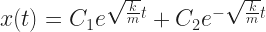
  , where ‘K’ is the ‘spring constant’. That’s some positive number again.


 , with C1 and C2 two possibly different numbers, and n1 and n2 two definitely different numbers. (If n1 and n2 were the same number then we should just add C1 and C2 together and stop using a more complicated expression than we need.) Remember that Newton’s Law of Motion about the sum of multiple forces being something vector something something direction? When we look at forces as potential energy functions, that law turns into just adding potential energies together. They’re well-behaved that way.
  . The little arrow above the symbol is one way to denote “this is a vector”. It’s a good scheme, what with arrows making people think of vectors and it being easy to write on a whiteboard. In books, sometimes, we make do just by putting the letter in boldface, L, which is easier for old-fashioned word processors to do. If we’re sure that the reader isn’t going to forget that L is this vector then we might stop highlighting the fact altogether. That’s even less work to do.
  , I know. Or, well, I know the story every physicist says about it. p is the designated letter for linear momentum because we used to use the word “impetus”, as in “impulse”, to mean what we mean by momentum these days. And “p” is the first letter in “impetus” that isn’t needed for some more urgent purpose. (“m” is too good a fit for mass. “i” has to work both as an index and as that number which, squared, gives us -1. And for that matter, “e” we need for that exponentials stuff, and “t” is too good a fit for time.) That said, while everybody, everybody, repeats this, I don’t know the source. Perhaps it is true. I can imagine, say, Euler or Lagrange in their writing settling on “p” for momentum and everybody copying them. I just haven’t seen a primary citation showing this is so.


