I mentioned in my last Reading the Comics post that it seems there are fewer mathematics-themed comic strips than there used to be. I know part of this is I’m trying to be more stringent. You don’t need me to say every time there’s a Roman numerals joke or that blackboards get mathematics symbols put on them. Still, it does feel like there’s fewer candidate strips. Maybe the end of the 2010s was a boom time for comic strips aimed at high school teachers and I only now appreciate that? Only further installments of this feature will let us know.
Jim Benton’s Jim Benton Cartoons for the 18th of April, 2022 suggests an origin for those famous overlapping circle pictures. This did get me curious what’s known about how John Venn came to draw overlapping circles. There’s no reason he couldn’t have used triangles or rectangles or any shape, after all. It looks like the answer is nobody really knows.
Venn, himself, didn’t name the diagrams after himself. Wikipedia credits Charles Dodgson (Lewis Carroll) as describing “Venn’s Method of Diagrams” in 1896. Clarence Irving Lewis, in 1918, seems to be the first person to write “Venn Diagram”. Venn wrote of them as “Eulerian Circles”, referencing the Leonhard Euler who just did everything. Sir William Hamilton — the philosopher, not the quaternions guy — posthumously published the Lectures On Metaphysics and Logic which used circles in these diagrams. Hamilton asserted, correctly, that you could use these to represent logical syllogisms. He wrote that the 1712 logic text Nucleus Logicae Weisianae — predating Euler — used circles, and was right about that. He got the author wrong, crediting Christian Weise instead of the correct author, Johann Christian Lange.
With 1712 the trail seems to end to this lay person doing a short essay’s worth of research. I don’t know what inspired Lange to try circles instead of any other shape. My guess, unburdened by evidence, is that it’s easy to draw circles, especially back in the days when every mathematician had a compass. I assume they weren’t too hard to typeset, at least compared to the many other shapes available. And you don’t need to even think about setting them with a rotation, the way a triangle or a pentagon might demand. But I also would not rule out a notion that circles have some connotation of perfection, in having infinite axes of symmetry and all points on them being equal in distance from the center and such. Might be the reasons fit in the intersection of the ethereal and the mundane.
Daniel Beyer’s Long Story Short for the 29th of April, 2022 puts out a couple of concepts from mathematical physics. These are all about geometry, which we now see as key to understanding physics. Particularly cosmology. The no-boundary proposal is a model constructed by James Hartle and Stephen Hawking. It’s about the first seconds of the universe after the Big Bang. This is an era that was so hot that all our well-tested models of physical law break down. The salient part of the Hartle-Hawking proposal is the idea that in this epoch time becomes indistinguishable from space. If I follow it — do not rely on my understanding for your thesis defense — it’s kind of the way that stepping away from the North Pole first creates the ideas of north and south and east and west. It’s very hard to think of a way to test this which would differentiate it from other hypotheses about the first instances of the universe.
The Weyl Curvature is a less hypothetical construct. It’s a tensor, one of many interesting to physicists. This one represents the tidal forces on a body that’s moving along a geodesic. So, for example, how the moon of a planet gets distorted over its orbit. The Weyl Curvature also offers a way to describe how gravitational waves pass through vacuum. I’m not aware of any serious question of the usefulness or relevance of the thing. But the joke doesn’t work without at least two real physics constructs as setup.
Liniers’ Macanudo for the 5th of May, 2022 has one of the imps who inhabit the comic asserting responsibility for making mathematics work. It’s difficult to imagine what a creature could do to make mathematics work, or to not work. If pressed, we would say mathematics is the set of things we’re confident we could prove according to a small, pretty solid-seeming set of logical laws. And a somewhat larger set of axioms and definitions. (Few of these are proved completely, but that’s because it would involve a lot of fiddly boring steps that nobody doubts we could do if we had to. If this sounds sketchy, consider: do you believe my claim that I could alphabetize the books on the shelf to my right, even though I’ve never done that specific task? Why?) It would be like making a word-search puzzle not work.
The punch line, the blue imp counting seventeen of the orange imp, suggest what this might mean. Mathematics as a set of statements following some rule, is a niche interest. What we like is how so many mathematical things seem to correspond to real-world things. We can imagine mathematics breaking that connection to the real world. The high temperature rising one degree each day this week may tell us something about this weekend, but it’s useless for telling us about November. So I can imagine a magical creature deciding what mathematical models still correspond to the thing they model. Be careful in trying to change their mind.
And that’s as many comic strips from the last several weeks that I think merit discussion. All of my Reading the Comics posts should be at this link, though. And I hope to have a new one again sometime soon. I’ll ask my contacts with the cartoonists. I have about half of a contact.
Mr Wu, my Singapore Maths Tuition friend, has offered many fine ideas for A-to-Z topics. This week’s is another of them, and I’m grateful for it.
Ordinary Differential Equations
As a rule, if you can do something with a number, you can do the same thing with a function. Not always, of course, but the exceptions are fewer than you might imagine. I’ll start with one of those things you can do to both.
A powerful thing we learn in (high school) algebra is that we can use a number without knowing what it is. We give it a name like ‘x’ or ‘y’ and describe what we find interesting about it. If we want to know what it is, we (usually) find some equation or set of equations and find what value of x could make that true. If we study enough (college) mathematics we learn its equivalent in functions. We give something a name like f or g or Ψ and describe what we know about it. And then try to find functions which make that true.
There are a couple common types of equation for these not-yet-known functions. The kind you expect to learn as a mathematics major involves differential equations. These are ones where your equation (or equations) involve derivatives of the not-yet-known f. A derivative describes the rate at which something changes. If we imagine the original f is a position, the derivative is velocity. Derivatives can have derivatives also; this second derivative would be the acceleration. And then second derivatives can have derivatives also, and so on, into infinity. When an equation involves a function and its derivatives we have a differential equation.
(The second common type is the integral equation, using a function and its integrals. And a third involves both derivatives and integrals. That’s known as an integro-differential equation, and isn’t life complicated enough? )
Differential equations themselves naturally divide into two kinds, ordinary and partial. They serve different roles. Usually an ordinary differential equation we can describe the change for from knowing only the current situation. (This may include velocities and accelerations and stuff. We could ask what the velocity at an instant means. But never mind that here.) Usually a partial differential equation bases the change where you are on the neighborhood of where your location. If you see holes you can pick in that, you’re right. The precise difference is about the independent variables. If the function f has more than one independent variable, it’s possible to take a partial derivative. This describes how f changes if one variable changes while the others stay fixed. If the function f has only the one independent variable, you can only take ordinary derivatives. So you get an ordinary differential equation.
But let’s speak casually here. If what you’re studying can be fully represented with a dashboard readout? Like, an ordered list of positions and velocities and stuff? You probably have an ordinary differential equation. If you need a picture with a three-dimensional surface or a color map to understand it? You probably have a partial differential equation.
One more metaphor. If you can imagine the thing you’re modeling as a marble rolling around on a hilly table? Odds are that’s an ordinary differential equation. And that representation covers a lot of interesting problems. Marbles on hills, obviously. But also rigid pendulums: we can treat the angle a pendulum makes and the rate at which those change as dimensions of space. The pendulum’s swinging then matches exactly a marble rolling around the right hilly table. Planets in space, too. We need more dimensions — three space dimensions and three velocity dimensions — for each planet. So, like, the Sun-Earth-and-Moon would be rolling around a hilly table with 18 dimensions. That’s all right. We don’t have to draw it. The mathematics works about the same. Just longer.
[ To be precise we need three momentum dimensions for each orbiting body. If they’re not changing mass appreciably, and not moving too near the speed of light, velocity is just momentum times a constant number, so we can use whichever is easier to visualize. ]
We mostly work with ordinary differential equations of either the first or the second order. First order means we have first derivatives in the equation, but never have to deal with more than the original function and its first derivative. Second order means we have second derivatives in the equation, but never have to deal with more than the original function or its first or second derivatives. You’ll never guess what a “third order” differential equation is unless you have experience in reading words. There are some reasons we stick to these low orders like first and second, though. One is that we know of good techniques for solving most first- and second-order ordinary differential equations. For higher-order differential equations we often use techniques that find a related normal old polynomial. Its solution helps with the thing we want. Or we break a high-order differential equation into a set of low-order ones. So yes, again, we search for answers where the light is good. But the good light covers many things we like to look at.
There’s simple harmonic motion, for example. It covers pendulums and springs and perturbations around stable equilibriums and all. This turns out to cover so many problems that, as a physics major, you get a little sick of simple harmonic motion. There’s the Airy function, which started out to describe the rainbow. It turns out to describe particles trapped in a triangular quantum well. The van der Pol equation, about systems where a small oscillation gets energy fed into it while a large oscillation gets energy drained. All kinds of exponential growth and decay problems. Very many functions where pairs of particles interact.
This doesn’t cover everything we would like to do. That’s all right. Ordinary differential equations lend themselves to numerical solutions. It requires considerable study and thought to do these numerical solutions well. But this doesn’t make the subject unapproachable. Few of us could animate the “Pink Elephants on Parade” scene from Dumbo. But could you draw a flip book of two stick figures tossing a ball back and forth? If you’ve had a good rest, a hearty breakfast, and have not listened to the news yet today, so you’re in a good mood?
The flip book ball is a decent example here, too. The animation will look good if the ball moves about the “right” amount between pages. A little faster when it’s first thrown, a bit slower as it reaches the top of its arc, a little faster as it falls back to the catcher. The ordinary differential equation tells us how fast our marble is rolling on this hilly table, and in what direction. So we can calculate how far the marble needs to move, and in what direction, to make the next page in the flip book.
Almost. The rate at which the marble should move will change, in the interval between one flip-book page and the next. The difference, the error, may not be much. But there is a difference between the exact and the numerical solution. Well, there is a difference between a circle and a regular polygon. We have many ways of minimizing and estimating and controlling the error. Doing that is what makes numerical mathematics the high-paid professional industry it is. Our game of catch we can verify by flipping through the book. The motion of four dozen planets and moons attracting one another is harder to be sure we calculate it right.
I said at the top that most anything one can do with numbers one can do with functions also. I would like to close the essay with some great parallel. Like, the way that trying to solve cubic equations made people realize complex numbers were good things to have. I don’t have a good example like that for ordinary differential equations, where the study expanded our ideas of what functions could be. Part of that is that complex numbers are more accessible than the stranger functions. Part of that is that complex numbers have a story behind them. The story features titanic figures like Gerolamo Cardano, Niccolò Tartaglia and Ludovico Ferrari. We see some awesome and weird personalities in 19th century mathematics. But their fights are generally harder to watch from the sidelines and cheer on. And part is that it’s easier to find pop historical treatments of the kinds of numbers. The historiography of what a “function” is is a specialist occupation.
But I can think of a possible case. A tool that’s sometimes used in solving ordinary differential equations is the “Dirac delta function”. Yes, that Paul Dirac. It’s a weird function, written as . It’s equal to zero everywhere, except where is zero. When is zero? It’s … we don’t talk about what it is. Instead we talk about what it can do. The integral of that Dirac delta function times some other function can equal that other function at a single point. It strains credibility to call this a function the way we speak of, like, or being functions. Many will classify it as a distribution instead. But it is so useful, for a particular kind of problem, that it’s impossible to throw away.
So perhaps the parallels between numbers and functions extend that far. Ordinary differential equations can make us notice kinds of functions we would not have seen otherwise.
And with this — I can see the much-postponed end of the Little 2021 Mathematics A-to-Z! You can read all my entries for 2021 at this link, and if you’d like can find all my A-to-Z essays here. How will I finish off the shortest yet most challenging sequence I’ve done yet? Will it be yellow and equivalent to the Axiom of Choice? Answers should come, in a week, if all starts going well.
And now, finally, I resume and hopefully finish what was meant to be a simpler and less stressful A-to-Z for last year. I’m feeling much better about my stress loads now and hope that I can soon enjoy the feeling of having a thing accomplished.
This topic is one of many suggestions that Elkement, one of my longest blog-friendships here, offered. It’s a creation that sent me back to my grad school textbooks, some of those slender paperback volumes with tiny, close-set type that turn out to be far more expensive than you imagine. Though not in this case: my most useful reference here was V I Arnold’s Ordinary Differential Equations, stamped inside as costing $18.75. The field is full of surprises. Another wonderful reference was this excellent set of notes prepared by Jodin Morey. They would have done much to help me through that class.
Tangent Space
Stand in midtown Manhattan, holding a map of midtown Manhattan. You have — not a tangent space, not yet. A tangent plane, representing the curved surface of the Earth with the flat surface of your map, though. But the tangent space is near: see how many blocks you must go, along the streets and the avenues, to get somewhere. Four blocks north, three west. Two blocks south, ten east. And so on. Those directions, of where you need to go, are the tangent space around you.
There is the first trick in tangent spaces. We get accustomed, early in learning calculus, to think of tangent lines and then of tangent planes. These are nice, flat approximations to some original curve. But while we’re introduced to the tangent space, and first learn examples of it, as tangent planes, we don’t stay there. There are several ways to define tangent spaces. One recasts tangent spaces in group theory terms, describing them as a ring based on functions that are equal to zero at the tangent point. (To be exact, it’s an ideal, based on a quotient group, based on two sets of such functions.)
That’s a description mathematicians are inclined to like, not only because it’s far harder to imagine than a map of the city is. But this ring definition describes the tangent space in terms of what we can do with it, rather than how to calculate finding it. That tends to appeal to mathematicians. And it offers surprising insights. Cleverer mathematicians than I am notice how this makes tangent spaces very close to Lagrange multipliers. Lagrange multipliers are a technique to find the maximum of a function subject to a constraint from another function. They seem to work by magic, and tangent spaces will echo that.
I’ll step back from the abstraction. There’s relevant observations to make from this map of midtown. The directions “four blocks north, three west” do not represent any part of Manhattan. It describes a way you might move in Manhattan, yes. But you could move in that direction from many places in the city. And you could go four blocks north and three west if you were in any part of any city with a grid of streets. It is a vector space, with elements that are velocities at a tangent point.
The tangent space is less a map showing where things are and more one of how to get to other places, closer to a subway map than a literal one. Still, the topic is steeped in the language of maps. I’ll find it a useful metaphor too. We do not make a map unless we want to know how to find something. So the interesting question is what do we try to find in these tangent spaces?
There are several routes to tangent spaces. The one I’m most familiar with is through dynamical systems. These are typically physics-driven, sometimes biology-driven, problems. They describe things that change in time according to ordinary differential equations. Physics problems particularly are often about things moving in space. Space, in dynamical systems, becomes “phase space”, an abstract universe spanned by all of the possible values of the variables. The variables are, usually, the positions and momentums of the particles (for a physics problem). Sometimes time and energy appear as variables. In biology variables are often things that represent populations. The role the Earth served in my first paragraph is now played by a manifold. The manifold represents whatever constraints are relevant to the problem. That’s likely to be conservation laws or limits on how often arctic hares can breed or such.
The evolution in time of this system, though, is now the tracing out of a path in phase space. An understandable and much-used system is the rigid pendulum. A stick, free to swing around a point. There are two useful coordinates here. There’s the angle the stick makes, relative to the vertical axis, . And there’s how fast the stick is changing, . You can draw these axes; I recommend as the horizontal and as the vertical axis but, you know, you do you.
If you give the pendulum a little tap, it’ll swing back and forth. It rises and moves to the right, then falls while moving to the left, then rises and moves to the left, then falls and moves to the right. In phase space, this traces out an ellipse. It’s your choice whether it’s going clockwise or anticlockwise. If you give the pendulum a huge tap, it’ll keep spinning around and around. It’ll spin a little slower as it gets nearly upright, but it speeds back up again. So in phase space that’s a wobbly line, moving either to the right or the left, depending what direction you hit it.
You can even imagine giving the pendulum just the right tap, exactly hard enough that it rises to vertical and balances there, perfectly aligned so it doesn’t fall back down. This is a special path, the dividing line between those ellipses and that wavy line. Or setting it vertically there to start with and trusting no truck driving down the street will rattle it loose. That’s a very precise dot, where is exactly zero. These paths, the trajectories, match whatever walking you did in the first paragraph to get to some spot in midtown Manhattan. And now let’s look again at the map, and the tangent space.
Within the tangent space we see what changes would change the system’s behavior. How much of a tap we would need, say, to launch our swinging pendulum into never-ending spinning. Or how much of a tap to stop a spinning pendulum. Every point on a trajectory of a dynamical system has a tangent space. And, for many interesting systems, the tangent space will be separable into two pieces. One of them will be perturbations that don’t go far from the original trajectory. One of them will be perturbations that do wander far from the original.
These regions may have a complicated border, with enclaves and enclaves within enclaves, and so on. This can be where we get (deterministic) chaos from. But what we usually find interesting is whether the perturbation keeps the old behavior intact or destroys it altogether. That is, how we can change where we are going.
That said, in practice, mathematicians don’t use tangent spaces to send pendulums swinging. They tend to come up when one is past studying such petty things as specific problems. They’re more often used in studying the ways that dynamical systems can behave. Tangent spaces themselves often get wrapped up into structures with names like tangent bundles. You’ll see them proving the existence of some properties, describing limit points and limit cycles and invariants and quite a bit of set theory. These can take us surprising places. It’s possible to use a tangent-space approach to prove the fundamental theorem of algebra, that every polynomial has at least one root. This seems to me the long way around to get there. But it is amazing to learn that is a place one can go.
I suspect it is impossible to say enough about Zeno’s Paradoxes. To close out my 2019 A-to-Z, though, I tried saying something. There are four particularly famous paradoxes and I discuss what are maybe the second and third-most-popular ones here. (The paradox of the Dichotomy is surely most famous.) The problems presented are about motion and may seem to be about physics, or at least about perception. But calculus is built on differentials, on the idea that we can describe how fast a thing is changing at an instant. Mathematicians have worked out a way to define this that we’re satisfied with and that doesn’t require (obvious) nonsense. But to claim we’ve solved Zeno’s Paradoxes — as unwary STEM majors sometimes do — is unwarranted.
Also I was able to work in a picture from an amusement park trip I took, the closing weekend of Kings Island park in 2019 and the last day that The Vortex roller coaster would run.
Today’s A To Z term was nominated by Dina Yagodich, who runs a YouTube channel with a host of mathematics topics. Zeno’s Paradoxes exist in the intersection of mathematics and philosophy. Mathematics majors like to declare that they’re all easy. The Ancient Greeks didn’t understand infinite series or infinitesimals like we do. Now they’re no challenge at all. This reflects a belief that philosophers must be silly people who haven’t noticed that one can, say, exit a room.
This is your classic STEM-attitude of missing the point. We may suppose that Zeno of Elea occasionally exited rooms himself. That is a supposition, though. Zeno, like most philosophers who lived before Socrates, we know from other philosophers making fun of him a century after he died. Or at least trying to explain what they thought he was on about. Modern philosophers are expected to present others’ arguments as well and as strongly as possible. This even — especially — when describing an argument they want to say is the stupidest thing they ever heard. Or, to use the lingo, when they wish to refute it. Ancient philosophers had no such compulsion. They did not mind presenting someone else’s argument sketchily, if they supposed everyone already knew it. Or even badly, if they wanted to make the other philosopher sound ridiculous. Between that and the sparse nature of the record, we have to guess a bit about what Zeno precisely said and what he meant. This is all right. We have some idea of things that might reasonably have bothered Zeno.
And they have bothered philosophers for thousands of years. They are about change. The ones I mean to discuss here are particularly about motion. And there are things we do not understand about change. This essay will not answer what we don’t understand. But it will, I hope, show something about why that’s still an interesting thing to ponder.
When we capture a moment by photographing it we add lies to what we see. We impose a frame on its contents, discarding what is off-frame. We rip an instant out of its context. And that before considering how we stage photographs, making people smile and stop tilting their heads. We forgive many of these lies. The things excluded from or the moments around the one photographed might not alter what the photograph represents. Making everyone smile can convey the emotional average of the event in a way that no individual moment represents. Arranging people to stand in frame can convey the participation in the way a candid photograph would not.
But there remains the lie that a photograph is “a moment”. It is no such thing. We notice this when the photograph is blurred. It records all the light passing through the lens while the shutter is open. A photograph records an eighth of a second. A thirtieth of a second. A thousandth of a second. But still, some time. There is always the ghost of motion in a picture. If we do not see it, it is because our photograph’s resolution is too coarse. If we could photograph something with infinite fidelity we would see, even in still life, the wobbling of the molecules that make up a thing.
One of the many loops of Vortex, a roller coaster at Kings Island amusement park from 1987 to 2019. Taken by me the last day of the ride’s operation; this was one of the roller coaster’s runs after 7 pm, the close of the park the last day of the season.
Which implies something fascinating to me. Think of a reel of film. Here I mean old-school pre-digital film, the thing that’s a great strip of pictures, a new one shown 24 times per second. Each frame of film is a photograph, recording some split-second of time. How much time is actually in a film, then? How long, cumulatively, was a camera shutter open during a two-hour film? I use pre-digital, strip-of-film movies for convenience. Digital films offer the same questions, but with different technical points. And I do not want the writing burden of describing both analog and digital film technologies. So I will stick to the long sequence of analog photographs model.
Let me imagine a movie. One of an ordinary everyday event; an actuality, to use the terminology of 1898. A person overtaking a walking tortoise. Look at the strip of film. There are many frames which show the person behind the tortoise. There are many frames showing the person ahead of the tortoise. When are the person and the tortoise at the same spot?
We have to put in some definitions. Fine; do that. Say we mean when the leading edge of the person’s nose overtakes the leading edge of the tortoise’s, as viewed from our camera. Or, since there must be blur, when the center of the blur of the person’s nose overtakes the center of the blur of the tortoise’s nose.
Do we have the frame when that moment happened? I’m sure we have frames from the moments before, and frames from the moments after. But the exact moment? Are you positive? If we zoomed in, would it actually show the person is a millimeter behind the tortoise? That the person is a hundredth of a millimeter ahead? A thousandth of a hair’s width behind? Suppose that our camera is very good. It can take frames representing as small a time as we need. Does it ever capture that precise moment? To the point that we know, no, it’s not the case that the tortoise is one-trillionth the width of a hydrogen atom ahead of the person?
If we can’t show the frame where this overtaking happened, then how do we know it happened? To put it in terms a STEM major will respect, how can we credit a thing we have not observed with happening? … Yes, we can suppose it happened if we suppose continuity in space and time. Then it follows from the intermediate value theorem. But then we are begging the question. We impose the assumption that there is a moment of overtaking. This does not prove that the moment exists.
Fine, then. What if time is not continuous? If there is a smallest moment of time? … If there is, then, we can imagine a frame of film that photographs only that one moment. So let’s look at its footage.
One thing stands out. There’s finally no blur in the picture. There can’t be; there’s no time during which to move. We might not catch the moment that the person overtakes the tortoise. It could “happen” in-between moments. But at least we have a moment to observe at leisure.
So … what is the difference between a picture of the person overtaking the tortoise, and a picture of the person and the tortoise standing still? A movie of the two walking should be different from a movie of the two pretending to be department store mannequins. What, in this frame, is the difference? If there is no observable difference, how does the universe tell whether, next instant, these two should have moved or not?
A mathematical physicist may toss in an answer. Our photograph is only of positions. We should also track momentum. Momentum carries within it the information of how position changes over time. We can’t photograph momentum, not without getting blurs. But analytically? If we interpret a photograph as “really” tracking the positions of a bunch of particles? To the mathematical physicist, momentum is as good a variable as position, and it’s as measurable. We can imagine a hyperspace photograph that gives us an image of positions and momentums. So, STEM types show up the philosophers finally, right?
Hold on. Let’s allow that somehow we get changes in position from the momentum of something. Hold off worrying about how momentum gets into position. Where does a change in momentum come from? In the mathematical physics problems we can do, the change in momentum has a value that depends on position. In the mathematical physics problems we have to deal with, the change in momentum has a value that depends on position and momentum. But that value? Put it in words. That value is the change in momentum. It has the same relationship to acceleration that momentum has to velocity. For want of a real term, I’ll call it acceleration. We need more variables. An even more hyperspatial film camera.
… And does acceleration change? Where does that change come from? That is going to demand another variable, the change-in-acceleration. (The “jerk”, according to people who want to tell you that “jerk” is a commonly used term for the change-in-acceleration, and no one else.) And the change-in-change-in-acceleration. Change-in-change-in-change-in-acceleration. We have to invoke an infinite regression of new variables. We got here because we wanted to suppose it wasn’t possible to divide a span of time infinitely many times. This seems like a lot to build into the universe to distinguish a person walking past a tortoise from a person standing near a tortoise. And then we still must admit not knowing how one variable propagates into another. That a person is wide is not usually enough explanation of how they are growing taller.
Numerical integration can model this kind of system with time divided into discrete chunks. It teaches us some ways that this can make logical sense. It also shows us that our projections will (generally) be wrong. At least unless we do things like have an infinite number of steps of time factor into each projection of the next timestep. Or use the forecast of future timesteps to correct the current one. Maybe use both. These are … not impossible. But being “ … not impossible” is not to say satisfying. (We allow numerical integration to be wrong by quantifying just how wrong it is. We call this an “error”, and have techniques that we can use to keep the error within some tolerated margin.)
So where has the movement happened? The original scene had movement to it. The movie seems to represent that movement. But that movement doesn’t seem to be in any frame of the movie. Where did it come from?
We can have properties that appear in a mass which don’t appear in any component piece. No molecule of a substance has a color, but a big enough mass does. No atom of iron is ferromagnetic, but a chunk might be. No grain of sand is a heap, but enough of them are. The Ancient Greeks knew this; we call it the Sorites paradox, after Eubulides of Miletus. (“Sorites” means “heap”, as in heap of sand. But if you had to bluff through a conversation about ancient Greek philosophers you could probably get away with making up a quote you credit to Sorites.) Could movement be, in the term mathematical physicists use, an intensive property? But intensive properties are obvious to the outside observer of a thing. We are not outside observers to the universe. It’s not clear what it would mean for there to be an outside observer to the universe. Even if there were, what space and time are they observing in? And aren’t their space and their time and their observations vulnerable to the same questions? We’re in danger of insisting on an infinite regression of “universes” just so a person can walk past a tortoise in ours.
We can say where movement comes from when we watch a movie. It is a trick of perception. Our eyes take some time to understand a new image. Our brains insist on forming a continuous whole story even out of disjoint ideas. Our memory fools us into remembering a continuous line of action. That a movie moves is entirely an illusion.
You see the implication here. Surely Zeno was not trying to lead us to understand all motion, in the real world, as an illusion? … Zeno seems to have been trying to support the work of Parmenides of Elea. Parmenides is another pre-Socratic philosopher. So we have about four words that we’re fairly sure he authored, and we’re not positive what order to put them in. Parmenides was arguing about the nature of reality, and what it means for a thing to come into or pass out of existence. He seems to have been arguing something like that there was a true reality that’s necessary and timeless and changeless. And there’s an apparent reality, the thing our senses observe. And in our sensing, we add lies which make things like change seem to happen. (Do not use this to get through your PhD defense in philosophy. I’m not sure I’d use it to get through your Intro to Ancient Greek Philosophy quiz.) That what we perceive as movement is not what is “really” going on is, at least, imaginable. So it is worth asking questions about what we mean for something to move. What difference there is between our intuitive understanding of movement and what logic says should happen.
(I know someone wishes to throw down the word Quantum. Quantum mechanics is a powerful tool for describing how many things behave. It implies limits on what we can simultaneously know about the position and the time of a thing. But there is a difference between “what time is” and “what we can know about a thing’s coordinates in time”. Quantum mechanics speaks more to the latter. There are also people who would like to say Relativity. Relativity, special and general, implies we should look at space and time as a unified set. But this does not change our questions about continuity of time or space, or where to find movement in both.)
And this is why we are likely never to finish pondering Zeno’s Paradoxes. In this essay I’ve only discussed two of them: Achilles and the Tortoise, and The Arrow. There are two other particularly famous ones: the Dichotomy, and the Stadium. The Dichotomy is the one about how to get somewhere, you have to get halfway there. But to get halfway there, you have to get a quarter of the way there. And an eighth of the way there, and so on. The Stadium is the hardest of the four great paradoxes to explain. This is in part because the earliest writings we have about it don’t make clear what Zeno was trying to get at. I can think of something which seems consistent with what’s described, and contrary-to-intuition enough to be interesting. I’m satisfied to ponder that one. But other people may have different ideas of what the paradox should be.
There are a handful of other paradoxes which don’t get so much love, although one of them is another version of the Sorites Paradox. Some of them the Stanford Encyclopedia of Philosophy dubs “paradoxes of plurality”. These ask how many things there could be. It’s hard to judge just what he was getting at with this. We know that one argument had three parts, and only two of them survive. Trying to fill in that gap is a challenge. We want to fill in the argument we would make, projecting from our modern idea of this plurality. It’s not Zeno’s idea, though, and we can’t know how close our projection is.
I don’t have the space to make a thematically coherent essay describing these all, though. The set of paradoxes have demanded thought, even just to come up with a reason to think they don’t demand thought, for thousands of years. We will, perhaps, have to keep trying again to fully understand what it is we don’t understand.
Thank you, all who’ve been reading, and who’ve offered topics, comments on the material, or questions about things I was hoping readers wouldn’t notice I was shorting. I’ll probably do this again next year, after I’ve had some chance to rest.
Of course I can’t just take a break for the sake of having a break. I feel like I have to do something of interest. So why not make better use of my several thousand past entries and repost one? I’d just reblog it except WordPress’s system for that is kind of rubbish. So here’s what I wrote, when I was first doing A-to-Z’s, back in summer of 2015. Somehow I was able to post three of these a week. I don’t know how.
I had remembered this essay as mostly describing the boring part of tensors, that we usually represent them as grids of numbers and then symbols with subscripts and superscripts. I’m glad to rediscover that I got at why we do such things to numbers and subscripts and superscripts.
Tensor.
The true but unenlightening answer first: a tensor is a regular, rectangular grid of numbers. The most common kind is a two-dimensional grid, so that it looks like a matrix, or like the times tables. It might be square, with as many rows as columns, or it might be rectangular.
It can also be one-dimensional, looking like a row or a column of numbers. Or it could be three-dimensional, rows and columns and whole levels of numbers. We don’t try to visualize that. It can be what we call zero-dimensional, in which case it just looks like a solitary number. It might be four- or more-dimensional, although I confess I’ve never heard of anyone who actually writes out such a thing. It’s just so hard to visualize.
You can add and subtract tensors if they’re of compatible sizes. You can also do something like multiplication. And this does mean that tensors of compatible sizes will form a ring. Of course, that doesn’t say why they’re interesting.
Tensors are useful because they can describe spatial relationships efficiently. The word comes from the same Latin root as “tension”, a hint about how we can imagine it. A common use of tensors is in describing the stress in an object. Applying stress in different directions to an object often produces different effects. The classic example there is a newspaper. Rip it in one direction and you get a smooth, clean tear. Rip it perpendicularly and you get a raggedy mess. The stress tensor represents this: it gives some idea of how a force put on the paper will create a tear.
Tensors show up a lot in physics, and so in mathematical physics. Technically they show up everywhere, since vectors and even plain old numbers (scalars, in the lingo) are kinds of tensors, but that’s not what I mean. Tensors can describe efficiently things whose magnitude and direction changes based on where something is and where it’s looking. So they are a great tool to use if one wants to represent stress, or how well magnetic fields pass through objects, or how electrical fields are distorted by the objects they move in. And they describe space, as well: general relativity is built on tensors. The mathematics of a tensor allow one to describe how space is shaped, based on how to measure the distance between two points in space.
My own mathematical education happened to be pretty tensor-light. I never happened to have courses that forced me to get good with them, and I confess to feeling intimidated when a mathematical argument gets deep into tensor mathematics. Joseph C Kolecki, with NASA’s Glenn (Lewis) Research Center, published in 2002 a nice little booklet “An Introduction to Tensors for Students of Physics and Engineering”. This I think nicely bridges some of the gap between mathematical structures like vectors and matrices, that mathematics and physics majors know well, and the kinds of tensors that get called tensors and that can be intimidating.
Mathematics is like every field in having jargon. Some jargon is unique to the field; there is no lay meaning of a “homeomorphism”. Some jargon is words plucked from the common language, such as “smooth”. The common meaning may guide you to what mathematicians want in it. A smooth function has a graph with no gaps, no discontinuities, no sharp corners; you can see smoothness in it. Sometimes the common meaning is an ambiguous help. A “series” is the sum of a sequence of numbers, that is, it is one number. Mathematicians study the series, but by looking at properties of the sequence.
So what sort of jargon is “atlas”? In common English, an atlas is a book of maps. Each map represents something different. Perhaps a different region of space. Perhaps a different scale, or a different projection altogether. The maps may show different features, or show them at different times. The maps must be about the same sort of thing. No slipping a map of Narnia in with the map of an amusement park, unless you warn of that in the title. The maps must not contradict one another. (So far as human-made things can be consistent, anyway.) And that’s the important stuff.
Atlas is the first kind of common-word jargon. Mathematicians use it to mean a collection of things. Those collected things aren’t mathematical maps. “Map” is the second type of jargon. The collected things are coordinate charts. “Coordinate chart” is a pairing of words not likely to appear in common English. But if you did encounter them? The meaning you might guess from their common use is not far off their mathematical use.
A coordinate chart is a matching of the points in an open set to normal coordinates. Euclidean coordinates, to be precise. But, you know, latitude and longitude, if it’s two dimensional. Add in the altitude if it’s three dimensions. Your x-y-z coordinates. It still counts if this is one dimension, or four dimensions, or sixteen dimensions. You’re less likely to draw a sketch of those. (In practice, you draw a sketch of a three-dimensional blob, and put N = 16 off in the corner, maybe in a box.)
These coordinate charts are on a manifold. That’s the second type of common-language jargon. Manifold, to pick the least bad of its manifold common definitions, is a “complicated object or subject”. The mathematical manifold is a surface. The things on that surface are connected by relationships that could be complicated. But the shape can be as simple as a plane or a sphere or a torus.
Every point on a coordinate chart needs some unique set of coordinates. And if a point appears on two coordinate charts, they have to be consistent. Consistent here is the matching between charts being a homeomorphism. A homeomorphism is a map, in the jargon sense. So it’s a function matching open sets on one chart to ope sets in the other chart. There’s more to it (there always is). But the important thing is that, away from the edges of the chart, we don’t create any new gaps or punctures or missing sections.
Some manifolds are easy to spot. The surface of the Earth, for example. Many are easy to come up with charts for. Think of any map of the Earth. Each point on the surface of the Earth matches some point on the sheet of paper. The coordinate chart is … let’s say how far your point is from the upper left corner of the page. (Pretend that you can measure those points precisely enough to match them to, like, the town you’re in.) Could be how far you are from the center, or the lower right corner, or whatever. These are all as good, and even count as other coordinate charts.
It’s easy to imagine that as latitude and longitude. We see maps of the world arranged by latitude and longitude so often. And that’s fine; latitude and longitude makes a good chart. But we have a problem in giving coordinates to the north and south pole. The latitude is easy but the longitude? So we have two points that can’t be covered on the map. We can save our atlas by having a couple charts. For the Earth this can be a map of most of the world arranged by latitude and longitude, and then two insets showing a disc around the north and the south poles. Thus we have an atlas of three charts.
We can make this a little tighter, reducing this to two charts. Have one that’s your normal sort of wall map, centered on the equator. Have the other be a transverse Mercator map. Make its center the great circle going through the prime meridian and the 180-degree antimeridian. Then every point on the planet, including the poles, has a neat unambiguous coordinate in at least one chart. A good chunk of the world will be on both charts. We can throw in more charts if we like, but two is enough.
The requirements to be an atlas aren’t hard to meet. So a lot of geometric structures end up being atlases. Theodore Frankel’s wonderful The Geometry of Physics introduces them on page 15. But that’s also the last appearance of “atlas”, at least in the index. The idea gets upstaged. The manifolds that the atlas charts end up being more interesting. Many problems about things in motion are easy to describe as paths traced out on manifolds. A large chunk of mathematical physics is then looking at this problem and figuring out what the space of possible behaviors looks like. What its topology is.
In a sense, the mathematical physicist might survey a problem, like a scout exploring new territory, more than solve it. This exploration brings us to directional derivatives. To tangent bundles. To other terms, jargon only partially informed by the common meanings.
This week’s topic is one of several suggested again by Mr Wu, blogger and Singaporean mathematics tutor. He’d suggested several topics, overlapping in their subject matter, and I was challenged to pick one.
Monte Carlo.
The reputation of mathematics has two aspects: difficulty and truth. Put “difficulty” to the side. “Truth” seems inarguable. We expect mathematics to produce sound, deductive arguments for everything. And that is an ideal. But we often want to know things we can’t do, or can’t do exactly. We can handle that often. If we can show that a number we want must be within some error range of a number we can calculate, we have a “numerical solution”. If we can show that a number we want must be within every error range of a number we can calculate, we have an “analytic solution”.
There are many things we’d like to calculate and can’t exactly. Many of them are integrals, which seem like they should be easy. We can represent any integral as finding the area, or volume, of a shape. The trick is that there’s only a few shapes with volumes we can find exact formulas for. You may remember the area of a triangle or a parallelogram. You have no idea what the area of a regular nonagon is. The trick we rely on is to approximate the shape we want with shapes we know formulas for. This usually gives us a numerical solution.
If you’re any bit devious you’ve had the impulse to think of a shape that can’t be broken up like that. There are such things, and a good swath of mathematics in the late 19th and early 20th centuries was arguments about how to handle them. I don’t mean to discuss them here. I’m more interested in the practical problems of breaking complicated shapes up into simpler ones and adding them all together.
One catch, an obvious one, is that if the shape is complicated you need a lot of simpler shapes added together to get a decent approximation. Less obvious is that you need way more shapes to do a three-dimensional volume well than you need for a two-dimensional area. That’s important because you need even way-er more to do a four-dimensional hypervolume. And more and more and more for a five-dimensional hypervolume. And so on.
That matters because many of the integrals we’d like to work out represent things like the energy of a large number of gas particles. Each of those particles carries six dimensions with it. Three dimensions describe its position and three dimensions describe its momentum. Worse, each particle has its own set of six dimensions. The position of particle 1 tells you nothing about the position of particle 2. So you end up needing ridiculously,impossibly many shapes to get even a rough approximation.
With no alternative, then, we try wisdom instead. We train ourselves to think of deductive reasoning as the only path to certainty. By the rules of deductive logic it is. But there are other unshakeable truths. One of them is randomness.
We can show — by deductive logic, so we trust the conclusion — that the purely random is predictable. Not in the way that lets us say how a ball will bounce off the floor. In the way that we can describe the shape of a great number of grains of sand dropped slowly on the floor.
The trick is one we might get if we were bad at darts. If we toss darts at a dartboard, badly, some will land on the board and some on the wall behind. How many hit the dartboard, compared to the total number we throw? If we’re as likely to hit every spot of the wall, then the fraction that hit the dartboard, times the area of the wall, should be about the area of the dartboard.
So we can do something equivalent to this dart-throwing to find the volumes of these complicated, hyper-dimensional shapes. It’s a kind of numerical integration. It isn’t particularly sensitive to how complicated the shape is, though. It takes more work to find the volume of a shape with more dimensions, yes. But it takes less more-work than the breaking-up-into-known-shapes method does. There are wide swaths of mathematics and mathematical physics where this is the best way to calculate the integral.
This bit that I’ve described is called “Monte Carlo integration”. The “integration” part of the name because that’s what we started out doing. To call it “Monte Carlo” implies either the method was first developed there or the person naming it was thinking of the famous casinos. The case is the latter. Monte Carlo methods as we know them come from Stanislaw Ulam, mathematical physicist working on atomic weapon design. While ill, he got to playing the game of Canfield solitaire, about which I know nothing except that Stanislaw Ulam was playing it in 1946 while ill. He wondered what the chance was that a given game was winnable. The most practical approach was sampling: set a computer to play a great many games and see what fractions of them were won. (The method comes from Ulam and John von Neumann. The name itself comes from their colleague Nicholas Metropolis.)
There are many Monte Carlo methods, with integration being only one very useful one. They hold in common that they’re build on randomness. We try calculations — often simple ones — many times over with many different possible values. And the regularity, the predictability, of randomness serves us. The results come together to an average that is close to the thing we do want to know.
Have a special one today. I’ve been reading a compilation of Crockett Johnson’s 1940s comic Barnaby. The title character, an almost too gentle child, follows his fairy godfather Mr O’Malley into various shenanigans. Many (the best ones, I’d say) involve the magical world. The steady complication is that Mr O’Malley boasts abilities beyond his demonstrated competence. (Although most of the magic characters are shown to be not all that good at their business.) It’s a gentle strip and everything works out all right, if farcically.
This particular strip comes from a late 1948 storyline. Mr O’Malley’s gone missing, coincidentally to a fairy cop come to arrest the pixie, who is a con artist at heart. So this sees the entry of Atlas, the Mental Giant, who’s got some pleasant gimmicks. One of them is his requiring mnemonics built on mathematical formulas to work out names. And this is a charming one, with a great little puzzle: how do you get A-T-L-A-S out of the formula Atlas has remembered?
Crockett Johnson and Jack Morley’s Barnaby for the 20th of December, 1948. (Morley drew the strip at this point.) I haven’t had cause to discuss other Barnaby strips but if I do, I’ll put them in an essay here. Sergeant Ausdauer reasons that “one of those upper-class amateur detectives with scientific minds who solve all the problems for Scotland Yard” could get him through this puzzle. If they were in London they could just ring any doorbell … which gives you a further sense of the comic strip’s sensibility.
I’m sorry the solution requires a bit of abusing notation, so please forgive it. But it’s a fun puzzle, especially as the joke would not be funnier if the formula didn’t work. I’m always impressed when a comic strip goes to that extra effort.
I have another mathematics-themed podcast to share. It’s again from the BBC’s In Our Time, a 50-minute program in which three experts discuss a topic. Here they came back around to mathematics and physics. And along the way chemistry and mensuration. The topic here was Pierre-Simon Laplace, who’s one of those people whose name you learn well as a mathematics or physics major. He doesn’t quite reach the levels of Euler — who does? — but he’s up there.
Laplace might be best known for his work in celestial mechanics. He (independently of Immanuel Kant) developed the nebular hypothesis, that the solar system formed from the contraction of a great cloud of dust. We today accept a modified version of this. And for studying the question of whether the solar system is stable. That is, whether the perturbations every planet has on one another average out to nothing, or to something catastrophic. And studying probability, which has more to do with these questions than one might imagine. And then there’s general mechanics, and differential equations, and if that weren’t enough, his role in establishing the Metric system. This and more gets discussion.
I’ve been reading The Disordered Cosmos: A Journey Into Dark Matter, Spacetime, and Dreams Deferred, by Chanda Prescod-Weinstein. It’s the best science book I’ve read in a long while.
Part of it is a pop-science discussion of particle physics and cosmology, as they’re now understood. It may seem strange that the tiniest things and the biggest thing are such natural companion subjects. That is what seems to make sense, though. I’ve fallen out of touch with a lot of particle physics since my undergraduate days and it’s wonderful to have it discussed well. This sort of pop physics is for me a pleasant comfort read.
The other part of the book is more memoir, and discussion of the culture of science. This is all discomfort reading. It’s an important discomfort.
I discuss sometimes how mathematics is, pretensions aside, a culturally-determined thing. Usually this is in the context of how, for example, that we have questions about “perfect numbers” is plausibly an idiosyncrasy. I don’t talk much about the culture of working mathematicians. In large part this is because I’m not a working mathematician, and don’t have close contact with working mathematicians. And then even if I did — well, I’m a tall, skinny white guy. I could step into most any college’s mathematics or physics department, sit down in a seminar, and be accepted as belonging there. People will assume that if I say anything, it’s worth listening to.
Chanda Prescod-Weinstein, a Black Jewish agender woman, does not get similar consideration. This despite her much greater merit. And, like, I was aware that women have it harder than men. And Black people have it harder than white people. And that being open about any but heterosexual cisgender inclinations is making one’s own life harder. What I hadn’t paid attention to was how much harder, and how relentlessly harder. Most every chapter, including the comfortable easy ones talking about families of quarks and all, is several needed slaps to my complacent face.
Her focus is on science, particularly physics. It’s not as though mathematics is innocent of driving women out or ignoring them when it can’t. Or of treating Black people with similar hostility. Much of what’s wrong is passively accepting patterns of not thinking about whether mathematics is open to everyone who wants in. Prescod-Weinstein offers many thoughts and many difficult thoughts. They are worth listening to.
I intend to post something inspired by the comics. I’m not ready just yet. Until then, though, I’d like to share a neat article published in Nature. It’s about paper.
The skeptical reader might say this is obvious. They’re invited to write a simulation that takes a set of fold lines and predicts which sides of the paper are angled out and which are angled in. The skeptical reader may also ask who cares about paper. It’s paper because many mathematics problems start from the kinds of things one sets one’s hands on. Anyone who’s seen a crack growing across their sidewalk, though — or across their countertop, or their grandfather’s desk — realizes there are things we don’t understand about how things break. And why they break that way. And, more generally, there’s a lot we don’t understand about how complicated “natural” shapes form. The big interest in this is how long molecules crumple up. The shapes of these govern how they behave, and it’d be nice to understand that more.
The problem I’d set out last week: I have a teapot good for about three cups of tea. I want to put milk in the once, before the first cup. How much should I drink before topping up the cup, to have the most milk at the end?
I have expectations. Some of this I know from experience, doing other problems where things get replaced at random. Here, tea or milk particles get swallowed at random, and replaced with tea particles. Yes, ‘particle’ is a strange word to apply to “a small bit of tea”. But it’s not like I can call them tea molecules. “Particle” will do and stop seeming weird someday.
Random replacement problems tend to be exponential decays. That I know from experience doing problems like this. So if I get an answer that doesn’t look like an exponential decay I’ll doubt it. I might be right, but I’ll need more convincing.
I also get some insight from extreme cases. We can call them reductios. Here “reductio” as in the word we usually follow with “ad absurdum”. Make the case ridiculous and see if that offers insight. The first reductio is to suppose I drink the entire first cup down to the last particle, then pour new tea in. By the second cup, there’s no milk left. The second reductio is to suppose I drink not a bit of the first cup of milk-with-tea. Then I have the most milk preserved. It’s not a satisfying break. But it leads me to suppose the most milk makes it through to the end if I have a lot of small sips and replacements of tea. And to look skeptically if my work suggests otherwise.
So that’s what I expect. What actually happens? Here, I do a bit of reasoning. Suppose that I have a mug. It can hold up to 1 unit of tea-and-milk. And the teapot, which holds up to 2 more units of tea-and-milk. What units? For the mathematics, I don’t care.
I’m going to suppose that I start with some amount — call it — of milk. is some number between 0 and 1. I fill the cup up to full, that is, 1 unit of tea-and-milk. And I drink some amount of the mixture. Call the amount I drink . It, too, is between 0 and 1. After this, I refill the mug up to full, so, putting in units of tea. And I repeat this until I empty the teapot. So I can do this times.
I know you noticed that I’m short on tea here. The teapot should hold 3 units of tea. I’m only pouring out . I could be more precise by refilling the mug times. I’m also going to suppose that I refill the mug with amount of tea a whole number of times. This sounds necessarily true. But consider: what if I drank and re-filled three-quarters of a cup of tea each time? How much tea is poured that third time?
I make these simplifications for good reasons. They reduce the complexity of the calculations I do without, I trust, making the result misleading. I can justify it too. I don’t drink tea from a graduated cylinder. It’s a false precision to pretend I do. I drink (say) about half my cup and refill it. How much tea I get in the teapot is variable too. Also, I don’t want to do that much work for this problem.
In fact, I’m going to do most of the work of this problem with a single drawing of a square. Here it is.
You may protest that my tea is not layered so the milk is all on the bottom, and that I do not drink a vertical column from it. To this I say: how do you know how I drink my tea?
So! I start out with units of tea in the mixture. After drinking units of milk-and-tea, what’s left is units of milk in the mixture.
How about the second refill? The process is the same as the first refill. But where, before, there had been units of milk in the tea, now there are only units in. So that horizontal strip is a little narrower is all. The same reasoning applies and so, after the second refill, there’s milk in the mixture.
If you nodded to that, you’d agree that after the third refill there’s . And are pretty sure what happens at the fourth and fifth and so on. If you didn’t nod to that, it’s all right. If you’re willing to take me on faith we can continue. If you’re not, that’s good too. Try doing a couple drawings yourself and you may convince yourself. If not, I don’t know. Maybe try, like, getting six white and 24 brown beads, stir them up, take out four at random. Replace all four with brown beads and count, and do that several times over. If you’re short on beads, cut up some paper into squares and write ‘B’ and ‘W’ on each square.
But anyone comfortable with algebra can see how to reduce this. The amount of milk remaining after j refills is going to be
How many refills does it take to run out of tea? That we knew from above: it’s refills. So my last full mug of tea will have left in it
units of milk.
Anyone who does differential equations recognizes this. It’s the discrete approximation of the exponential decay curve. Discrete, here, because we take out some finite but nonzero amount of milk-and-tea, , and replace it with the same amount of pure tea.
Now, again, I’ve seen this before so I know its conclusions. The most milk will make it to the end of is as small as possible. The best possible case would be if I drink and replace an infinitesimal bit of milk-and-tea each time. Then the last mug would end with of milk. That’s as in the base of the natural logarithm. Every mathematics problem has an somewhere in it and I’m not exaggerating much. All told this would be about 13 and a half percent of the original milk.
Drinking more realistic amounts, like, half the mug before refilling, makes the milk situation more dire. Replacing half the mug at a time means the last full mug has only one-sixteenth what I started with. Drinking a quarter of the mug and replacing it lets about one-tenth the original milk survive.
But all told the lesson is clear. If I want milk in the last mug, I should put some in each refill. Putting all the milk in at the start and letting it dissolve doesn’t work.
A post on Mathstodon made me aware there’s a bit of talk about iceberg shapes. Particularly that one of the iconic photographs of an iceberg above-and-below water, is a imaginative work. A real iceberg wouldn’t be stable in that orientation. Which, I’ll admit, isn’t something I had thought about. I also hadn’t thought about the photography challenge of getting a clear picture of something in sunlight and in water at once. There was a lot I hadn’t thought about. In my defense, I spend a lot of time noticing comic strips had a character complain about the New Math.
But this all leads me to a fun little play tool: Iceberger, designed to let you sketch in a potential iceberg and see what it does. Often, that’s roll over to a more stable orientation. It’s fun to play with, and to watch shapes tilt over, gradually or rapidly. And playing with it may help one develop a sense for what kinds of shapes should be stable in water, and what kinds should not.
Rosenbluth was a PhD in physics (and an Olympics-qualified fencer). Her postdoctoral work was with the Atomic Energy Commission, bringing her to a position at Los Alamos National Laboratory in the early 1950s. And a moment in computer science that touches very many people’s work, my own included. This is in what we call Metropolis-Hastings Markov Chain Monte Carlo.
Monte Carlo methods are numerical techniques that rely on randomness. The name references the casinos. Markov Chain refers to techniques that create a sequence of things. Each thing exists in some set of possibilities. If we’re talking about Markov Chain Monte Carlo this is usually an enormous set of possibilities, too many to deal with by hand, except for little tutorial problems. The trick is that what the next item in the sequence is depends on what the current item is, and nothing more. This may sound implausible — when does anything in the real world not depend on its history? — but the technique works well regardless. Metropolis-Hastings is a way of finding states that meet some condition well. Usually this is a maximum, or minimum, of some interesting property. The Metropolis-Hastings rule has the chance of going to an improved state, one with more of whatever the property we like, be 1, a certainty. The chance of going to a worsened state, with less of the property, be not zero. The worse the new state is, the less likely it is, but it’s never zero. The result is a sequence of states which, most of the time, improve whatever it is you’re looking for. It sometimes tries out some worse fits, in the hopes that this leads us to a better fit, for the same reason sometimes you have to go downhill to reach a larger hill. The technique works quite well at finding approximately-optimum states when it’s hard to find the best state, but it’s easy to judge which of two states is better. Also when you can have a computer do a lot of calculations, because it needs a lot of calculations.
So here we come to Rosenbluth. She and her then-husband, according to an interview he gave in 2003, were the primary workers behind the 1953 paper that set out the technique. And, particularly, she wrote the MANIAC computer program which ran the algorithm. It’s important work and an uncounted number of mathematicians, physicists, chemists, biologists, economists, and other planners have followed. She would go on to study statistical mechanics problems, in particular simulations of molecules. It’s still a rich field of study.
This is easy. The velocity is the first derivative of the position. First derivative with respect to time, if you must know. That hardly needed an extra week to write.
Yes, there’s more. There is always more. Velocity is important by itself. It’s also important for guiding us into new ideas. There are many. One idea is that it’s often the first good example of vectors. Many things can be vectors, as mathematicians see them. But the ones we think of most often are “some magnitude, in some direction”.
The position of things, in space, we describe with vectors. But somehow velocity, the changes of positions, seems more significant. I suspect we often find static things below our interest. I remember as a physics major that my Intro to Mechanics instructor skipped Statics altogether. There are many important things, like bridges and roofs and roller coaster supports, that we find interesting because they don’t move. But the real Intro to Mechanics is stuff in motion. Balls rolling down inclined planes. Pendulums. Blocks on springs. Also planets. (And bridges and roofs and roller coaster supports wouldn’t work if they didn’t move a bit. It’s not much though.)
So velocity shows us vectors. Anything could, in principle, be moving in any direction, with any speed. We can imagine a thing in motion inside a room that’s in motion, its net velocity being the sum of two vectors.
And they show us derivatives. A compelling answer to “what does differentiation mean?” is “it’s the rate at which something changes”. Properly, we can take the derivative of any quantity with respect to any variable. But there are some that make sense to do, and position with respect to time is one. Anyone who’s tried to catch a ball understands the interest in knowing.
We take derivatives with respect to time so often we have shorthands for it, by putting a ‘ mark after, or a dot above, the variable. So if x is the position (and it often is), then is the velocity. If we want to emphasize we think of vectors, is the position and the velocity.
Velocity has another common shorthand. This is , or if we want to emphasize its vector nature, . Why a name besides the good enough ? It helps us avoid misplacing a ‘ mark in our work, for one. And giving velocity a separate symbol encourages us to think of the velocity as independent from the position. It’s not — not exactly — independent. But knowing that a thing is in the lawn outside tells us nothing about how it’s moving. Velocity affects position, in a process so familiar we rarely consider how there’s parts we don’t understand about it. But velocity is also somehow also free of the position at an instant.
Velocity also guides us into a first understanding of how to take derivatives. Thinking of the change in position over smaller and smaller time intervals gets us to the “instantaneous” velocity by doing only things we can imagine doing with a ruler and a stopwatch.
Velocity has a velocity. , also known as . Or, if we’re sure we won’t lose a ‘ mark, . Once we are comfortable thinking of how position changes in time we can think of other changes. Velocity’s change in time we call acceleration. This is also a vector, more abstract than position or velocity. Multiply the acceleration by the mass of the thing accelerating and we have a vector called the “force”. That, we at least feel we understand, and can work with.
Acceleration has a velocity too, a rate of change in time. It’s called the “jerk” by people telling you the change in acceleration in time is called the “jerk”. (I don’t see the term used in the wild, but admit my experience is limited.) And so on. We could, in principle, keep taking derivatives of the position and keep finding new changes. But most physics problems we find interesting use just a couple of derivatives of the position. We can label them, if we need, , where n is some big enough number like 4.
We can bundle them in interesting ways, though. Come back to that mention of treating position and velocity of something as though they were independent coordinates. It’s a useful perspective. Imagine the rules about how particles interacting with one another and with their environment. These usually have explicit roles for position and velocity. (Granting this may reflect a selection bias. But these do cover enough interesting problems to fill a career.)
So we create a new vector. It’s made of the positition and the velocity. We’d write it out as . The superscript-T there, “transposition”, lets us use the tools of matrix algebra. This vector describes a point in phase space. Phase space is the collection of all the physically possible positions and velocities for the system.
What’s the derivative, in time, of this point in phase space? Glad to say we can do this piece by piece. The derivative of a vector is the derivative of each component of a vector. So the derivative of is , or, . This acceleration itself depends on, normally, the positions and velocities. So we can describe this as for some function . You are surely impressed with this symbol-shuffling. You are less sure why this bother.
The bother is a trick of ordinary differential equations. All differential equations are about how a function-to-be-determined and its derivatives relate to one another. In ordinary differential equations, the function-to-be-determined depends on a single variable. Usually it’s called x or t. There may be many derivatives of f. This symbol-shuffling rewriting takes away those higher-order derivatives. We rewrite the equation as a vector equation of just one order. There’s some point in phase space, and we know what its velocity is. That we do because in this form many problems can be written as a matrix problem: . Or approximate our problem as a matrix problem. This lets us bring in linear algebra tools, and that’s worthwhile.
It also lets us bring in numerical tools. Numerical mathematics has developed many methods to solve the ordinary differential equation. Most of them extend to . The result is a classic mathematician’s trick. We can recast a problem as one we have better tools to solve.
It calls on a more abstract idea of what a “velocity” might be. We can explain what the thing that’s “moving” and what it’s moving through are, given time. But the instincts we develop from watching ordinary things move help us in these new territories. This is also a classic mathematician’s trick. It may seem like all mathematicians do is develop tricks to extend what they already do. I can’t say this is wrong.
I assume that last week I disappointed Mr Wu, of the Singapore Maths Tuition blog, last week when I passed on a topic he suggested to unintentionally rewrite a good enough essay. I hope to make it up this week with a piece of linear algebra.
A Unitary Matrix — note the article; there is not a singular the Unitary Matrix — starts with a matrix. This is an ordered collection of scalars. The scalars we call elements. I can’t think of a time I ever saw a matrix represented except as a rectangular grid of elements, or as a capital letter for the name of a matrix. Or a block inside a matrix. In principle the elements can be anything. In practice, they’re almost always either real numbers or complex numbers. To speak of Unitary Matrixes invokes complex-valued numbers. If a matrix that would be Unitary has only real-valued elements, we call that an Orthogonal Matrix. It’s not wrong to call an Orthogonal matrix “Unitary”. It’s like pointing to a known square, though, and calling it a parallelogram. Your audience will grant that’s true. But it wonder what you’re getting at, unless you’re talking about a bunch of parallelograms and some of them happen to be squares.
As with polygons, though, there are many names for particular kinds of matrices. The flurry of them settles down on the Intro to Linear Algebra student and it takes three or four courses before most of them feel like familiar names. I will try to keep the flurry clear. First, we’re talking about square matrices, ones with the same number of rows as columns.
Start with any old square matrix. Give it the name U because you see where this is going. There are a couple of new matrices we can derive from it. One of them is the complex conjugate. This is the matrix you get by taking the complex conjugate of every term. So, if one element is , in the complex conjugate, that element would be . Reverse the plus or minus sign of the imaginary component. The shorthand for “the complex conjugate to matrix U” is . Also we’ll often just say “the conjugate”, taking the “complex” part as implied.
Start back with any old square matrix, again called U. Another thing you can do with it is take the transposition. This matrix, U-transpose, you get by keeping the order of elements but changing rows and columns. That is, the elements in the first row become the elements in the first column. The elements in the second row become the elements in the second column. Third row becomes the third column, and so on. The diagonal — first row, first column; second row, second column; third row, third column; and so on — stays where it was. The shorthand for “the transposition of U” is .
You can chain these together. If you start with U and take both its complex-conjugate and its transposition, you get the adjoint. We write that with a little dagger: . For a wonder, as matrices go, it doesn’t matter whether you take the transpose or the conjugate first. It’s the same . You may ask how people writing this out by hand never mistake for . This is a good question and I hope to have an answer someday. (I would write it as in my notes.)
And the last thing you can maybe do with a square matrix is take its inverse. This is like taking the reciprocal of a number. When you multiply a matrix by its inverse, you get the Identity Matrix. Not every matrix has an inverse, though. It’s worse than real numbers, where only zero doesn’t have a reciprocal. You can have a matrix that isn’t all zeroes and that doesn’t have an inverse. This is part of why linear algebra mathematicians command the big money. But if a matrix U has an inverse, we write that inverse as .
The Identity Matrix is one of a family of square matrices. Every element in an identity matrix is zero, except on the diagonal. That is, the element at row one, column one, is the number 1. The element at row two, column two is also the number 1. Same with row three, column three: another one. And so on. This is the “identity” matrix because it works like the multiplicative identity. Pick any matrix you like, and multiply it by the identity matrix; you get the original matrix right back. We use the name for an identity matrix. If we have to be clear how many rows and columns the matrix has, we write that as a subscript: or or or so on.
So this, finally, lets me say what a Unitary Matrix is. It’s any square matrix U where the adjoint, is the same matrix as the inverse, . It’s wonderful to learn you have a Unitary Matrix. Not just because, most of the time, finding the inverse of a matrix is a long and tedious procedure. Here? You have to write the elements in a different order and change the plus-or-minus sign on the imaginary numbers. The only way it would be easier if you had only real numbers, and didn’t have to take the conjugates.
That’s all a nice heap of terms. What makes any of them important, other than so Intro to Linear Algebra professors can test their students?
Well, you know mathematicians. If we like something like this, it’s usually because it holds out the prospect of turning a hard problems into easier ones. So it is. Start out with any old matrix. Call it A. Then there exist some unitary matrixes, call them U and V. And their product does something wonderful: is a “diagonal” matrix. A diagonal matrix has zeroes for every element except the diagonal ones. That is, row one, column one; row two, column two; row three, column three; and so on. The elements that trace a path from the upper-left to the lower-right corner of the matrix. (The diagonal from the upper-right to the lower-left we have nothing to do with.) Everything we might do with matrices is easier on a diagonal matrix. So we process our matrix A into this diagonal matrix D. Process it by whatever the heck we’re doing. If we then multiply this by the inverses of U and V? If we calculate ? We get whatever our process would have given us had we done it to A. And, since U and V are unitary matrices, it’s easy to find these inverses. Wonderful!
Also this sounds like I just said Unitary Matrixes are great because they solve a problem you never heard of before.
The 20th Century’s first great use for Unitary Matrixes, and I imagine the impulse for Mr Wu’s suggestion, was quantum mechanics. (A later use would be data compression.) Unitary Matrixes help us calculate how quantum systems evolve. This should be a little easier to understand if I use a simple physics problem as demonstration.
So imagine three blocks, all the same mass. They’re connected in a row, left to right. There’s two springs, one between the left and the center mass, one between the center and the right mass. The springs have the same strength. The blocks can only move left-to-right. But, within those bounds, you can do anything you like with the blocks. Move them wherever you like and let go. Let them go with a kick moving to the left or the right. The only restraint is they can’t pass through one another; you can’t slide the center block to the right of the right block.
This is not quantum mechanics, by the way. But it’s not far, either. You can turn this into a fine toy of a molecule. For now, though, think of it as a toy. What can you do with it?
A bunch of things, but there’s two really distinct ways these blocks can move. These are the ways the blocks would move if you just hit it with some energy and let the system do what felt natural. One is to have the center block stay right where it is, and the left and right blocks swinging out and in. We know they’ll swing symmetrically, the left block going as far to the left as the right block goes to the right. But all these symmetric oscillations look about the same. They’re one mode.
The other is … not quite antisymmetric. In this mode, the center block moves in one direction and the outer blocks move in the other, just enough to keep momentum conserved. Eventually the center block switches direction and swings the other way. But the outer blocks switch direction and swing the other way too. If you’re having trouble imagining this, imagine looking at it from the outer blocks’ point of view. To them, it’s just the center block wobbling back and forth. That’s the other mode.
And it turns out? It doesn’t matter how you started these blocks moving. The movement looks like a combination of the symmetric and the not-quite-antisymmetric modes. So if you know how the symmetric mode evolves, and how the not-quite-antisymmetric mode evolves? Then you know how every possible arrangement of this system evolves.
So here’s where we get to quantum mechanics. Suppose we know the quantum mechanics description of a system at some time. This we can do as a vector. And we know the Hamiltonian, the description of all the potential and kinetic energy, for how the system evolves. The evolution in time of our quantum mechanics description we can see as a unitary matrix multiplied by this vector.
The Hamiltonian, by itself, won’t (normally) be a Unitary Matrix. It gets the boring name H. It’ll be some complicated messy thing. But perhaps we can find a Unitary Matrix U, so that is a diagonal matrix. And then that’s great. The original H is hard to work with. The diagonalized version? That one we can almost always work with. And then we can go from solutions on the diagonalized version back to solutions on the original. (If the function describes the evolution of , then describes the evolution of .) The work that U (and ) does to H is basically what we did with that three-block, two-spring model. It’s picking out the modes, and letting us figure out their behavior. Then put that together to work out the behavior of what we’re interested in.
There are other uses, besides time-evolution. For instance, an important part of quantum mechanics and thermodynamics is that we can swap particles of the same type. Like, there’s no telling an electron that’s on your nose from an electron that’s in one of the reflective mirrors the Apollo astronauts left on the Moon. If they swapped positions, somehow, we wouldn’t know. It’s important for calculating things like entropy that we consider this possibility. Two particles swapping positions is a permutation. We can describe that as multiplying the vector that describes what every electron on the Earth and Moon is doing by a Unitary Matrix. Here it’s a matrix that does nothing but swap the descriptions of these two electrons. I concede this doesn’t sound thrilling. But anything that goes into calculating entropy is first-rank important.
As with time-evolution and with permutation, though, any symmetry matches a Unitary Matrix. This includes obvious things like reflecting across a plane. But it also covers, like, being displaced a set distance. And some outright obscure symmetries too, such as the phase of the state function . I don’t have a good way to describe what this is, physically; we can’t observe it directly. This symmetry, though, manifests as the conservation of electric charge, a thing we rather like.
This, then, is the sort of problem that draws Unitary Matrixes to our attention.
I have again Elke Stangl, author of elkemental Force, to thank for the subject this week. Again, Stangl’s is a blog of wide-ranging theme interests. And it’s got more poetry this week again, this time haikus about the Dirac delta function.
I also have Kerson Huang, of the Massachusetts Institute of Technology and of Nanyang Technological University, to thank for much insight into the week’s subject. Huang published this A Critical History of Renormalization, which gave me much to think about. It’s likely a paper that would help anyone hoping to know the history of the technique better.
There is a mathematical model, the Ising Model, for how magnets work. The model has the simplicity of a toy model given by a professor (Wilhelm Lenz) to his grad student (Ernst Ising). Suppose matter is a uniform, uniformly-spaced grid. At each point on the grid we have either a bit of magnetism pointed up (value +1) or down (value -1). It is a nearest-neighbor model. Each point interacts with its nearest neighbors and none of the other points. For a one-dimensional grid this is easy. It’s the stuff of thermodynamics homework for physics majors. They don’t understand it, because you need the hyperbolic trigonometric functions. But they could. For two dimensions … it’s hard. But doable. And interesting. It describes important things like phase changes. The way that you can take a perfectly good strong magnet and heat it up until it’s an iron goo, then cool it down to being a strong magnet again.
For such a simple model it works well. A lot of the solids we find interesting are crystals, or are almost crystals. These are molecules arranged in a grid. So that part of the model is fine. They do interact, foremost, with their nearest neighbors. But not exclusively. In principle, every molecule in a crystal interacts with every other molecule. Can we account for this? Can we make a better model?
Yes, many ways. Here’s one. It’s designed for a square grid, the kind you get by looking at the intersections on a normal piece of graph paper. Each point is in a row and a column. The rows are a distance ‘a’ apart. So are the columns.
Now draw a new grid, on top of the old. Do it by grouping together two-by-two blocks of the original. Draw new rows and columns through the centers of these new blocks. Put at the new intersections a bit of magnetism. Its value is the mean of whatever the four blocks around it are. So, could be 1, could be -1, could be 0, could be ½, could be -½. There’s more options. But look at what we have. It’s still an Ising-like model, with interactions between nearest-neighbors. There’s more choices for what value each point can have. And the grid spacing is now 2a instead of a. But it all looks pretty similar.
And now the great insight, that we can trace to Leo P Kadanoff in 1966. What if we relabel the distance between grid points? We called it 2a before. Call it a, now, again. What’s important that’s different from the Ising model we started with?
There’s the not-negligible point that there’s five different values a point can have, instead of two. But otherwise? In the operations we do, not much is different. How about in what it models? And there it’s interesting. Think of the original grid points. In the original scaling, they interacted only with units one original-row or one original-column away. Now? Their average interacts with the average of grid points that were as far as three original-rows or three original-columns away. It’s a small change. But it’s closer to reflecting the reality of every molecule interacting with every other molecule.
You know what happens when mathematicians get one good trick. We figure what happens if we do it again. Take the rescaled grid, the one that represents two-by-two blocks of the original. Rescale it again, making two-by-two blocks of these two-by-two blocks. Do the same rules about setting the center points as a new grid. And then re-scaling. What we have now are blocks that represent averages of four-by-four blocks of the original. And that, imperfectly, let a point interact with a point seven original-rows or original-columns away. (Or farther: seven original-rows down and three original-columns to the left, say. Have fun counting all the distances.) And again: we have eight-by-eight blocks and even more range. Again: sixteen-by-sixteen blocks and double the range again. Why not carry this on forever?
This is renormalization. It’s a specific sort, called the block-spin renormalization group. It comes from condensed matter physics, where we try to understand how molecules come together to form bulks of matter. Kenneth Wilson stretched this over to studying the Kondo Effect. This is a problem in how magnetic impurities affect electrical resistance. (It’s named for Jun Kondo.) It’s great work. It (in part) earned Wilson a Nobel Prize. But the idea is simple. We can understand complex interactions by making them simple ones. The interactions have a natural scale, cutting off at the nearest neighbor. But we redefine ‘nearest neighbor’, again and again, until it reaches infinitely far away.
This problem, and its solution, come from thermodynamics. Particularly, statistical mechanics. This is a bit ahistoric. Physicists first used renormalization in quantum mechanics. This is all right. As a general guideline, everything in statistical mechanics turns into something in quantum mechanics, and vice-versa. What quantum mechanics lacked, for a generation, was logical rigor for renormalization. This statistical mechanics approach provided that.
Renormalization in quantum mechanics we needed because of virtual particles. Quantum mechanics requires that particles can pop into existence, carrying momentum, and then pop back out again. This gives us electromagnetism, and the strong nuclear force (which holds particles together), and the weak nuclear force (which causes nuclear decay). Leave gravity over on the side. The more momentum in the virtual particle, the shorter a time it can exist. It’s actually the more energy, the shorter the particle lasts. In that guise you know it as the Uncertainty Principle. But it’s momentum that’s important here. This means short-range interactions transfer more momentum, and long-range ones transfer less. And here we had thought forces got stronger as the particles interacting got closer together.
In principle, there is no upper limit to how much momentum one of these virtual particles can have. And, worse, the original particle can interact with its virtual particle. This by exchanging another virtual particle. Which is even higher-energy and shorter-range. The virtual particle can also interact with the field that’s around the original particle. Pairs of virtual particles can exchange more virtual particles. And so on. What we get, when we add this all together, seems like it should be infinitely large. Every particle the center of an infinitely great bundle of energy.
Renormalization, the original renormalization, cuts that off. Sets an effective limit on the system. The limit is not “only particles this close will interact” exactly. It’s more “only virtual particles with less than this momentum will”. (Yes, there’s some overlap between these ideas.) This seems different to us mere dwellers in reality. But to a mathematical physicist, knowing that position and momentum are conjugate variables? Limiting one is the same work as limiting the other.
This, when developed, left physicists uneasy. It’s for good reasons. The cutoff is arbitrary. Its existence, sure, but we often deal with arbitrary cutoffs for things. When we calculate a weather satellite’s orbit we do not care that other star systems exist. We barely care that Jupiter exists. Still, where to put the cutoff? Quantum Electrodynamics, using this, could provide excellent predictions of physical properties. But shouldn’t we get different predictions with different cutoffs? How do we know we’re not picking a cutoff because it makes our test problem work right? That we’re not picking one that produces garbage for every other problem? Read the writing of a physicist of the time and — oh, why be coy? We all read Richard Feynman, his QED at least. We see him sulking about a technique he used to brilliant effect.
Wilson-style renormalization answered Feynman’s objections. (Though not to Feynman’s satisfaction, if I understand the history right.) The momentum cutoff serves as a scale. Or if you prefer, the scale of interactions we consider tells us the cutoff. Different scales give us different quantum mechanics. One scale, one cutoff, gives us the way molecules interact together, on the scale of condensed-matter physics. A different scale, with a different cutoff, describes the particles of Quantum Electrodynamics. Other scales describe something more recognizable as classical physics. Or the Yang-Mills gauge theory, as describes the Standard Model of subatomic particles, all those quarks and leptons.
Renormalization offers a capsule of much of mathematical physics, though. It started as an arbitrary trick to avoid calculation problems. In time, we found a rationale for the trick. But found it from looking at a problem that seemed unrelated. On learning the related trick well, though, we see they’re different aspects of the same problem. It’s a neat bit of work.
This is the 141st Playful Math Education Blog Carnival. And I will be taking this lower-key than I have past times I was able to host the carnival. I do not have higher keys available this year.
The Numbers
I will start by borrowing a page from Iva Sallay, kind creator and host of FindTheFactors.com, and say some things about 141. I owe Iva Sallay many things, including this comfortable lead-in to the post, and my participation in the Playful Math Education Blog Carnival. She was also kind enough to send me many interesting blogs and pages and I am grateful.
141 is a centered pentagonal number. It’s like 1 or 6 or 16 that way. That is, if I give you six pennies and ask you to do something with it, a natural thing is one coin in the center and a pentagon around that. With 16 coins, you can add a nice regular pentagon around that, one that reaches three coins from vertex to vertex. 31, 51, 76, and 106 are the next couple centered pentagonal numbers. 181 and 226 are the next centered pentagonal numbers. The units number in these follow a pattern, too, in base ten. The last digits go 1-6-6-1, 1-6-6-1, 1-6-6-1, and so on.
141’s also a hendecagonal number. That is, arrange your coins to make a regular 11-sided polygon. 1 and then 11 are hendecagonal numbers. Then 30, 58, 95, and 141. 196 and 260 are the next couple. There are many of these sorts of polygonal numbers, for any regular polygon you like.
141 is also a Hilbert Prime, a class of number I hadn’t heard of before. It’s still named for the Hilbert of Hilbert’s problems. 141 is not a prime number, which you notice from adding up the digits. But a Hilbert Prime is a different kind of beast. These come from looking at counting numbers that are one more than a whole multiple of four. So, numbers like 1, 5, 9, 13, and so on. This sequence describes a lot of classes of numbers. A Hilbert Prime, at least as some number theorists use it, is a Hilbert Number that can’t be divided by any other Hilbert Number (other than 1). So these include 5, 9, 13, 17, and 21, and some of those are already not traditional primes. There are Hilbert Numbers that are the products of different sets of Hilbert Primes, such as 441 or 693. (441 is both 21 times 21 and also 9 times 49. 693 is 9 times 77 and also 21 times 33) So I don’t know what use Hilbert Primes are specifically. If someone knows, I’d love to hear.
Second round of overflow parking at Dorney Park. From a visit we took in August of 2014, you remember, that day everybody in eastern Pennsylvania, north Jersey, and southern New York State decided to go to Dorney Park. All these amusement park pictures are ones I’ve taken and I’m happy to say, truthfully, that they’re all connected to something in the main text.
Also, at the risk of causing trouble, The Aperiodical also hosts a monthly Carnival of Mathematics. It’s a similar gathering of interesting mathematics content. It doesn’t look necessarily for educational or playful pieces.
The Reflective Educator posted Precision In Language. This is about one of the hardest bits of teaching. That is to say things which are true and which can’t be mis-remembered as something false. Author David Wees points out an example of this hazard, as kids apply rules outside their context.
Simon Gregg’s essay The Gardener and the Carpenter follows a connected theme. The experience students have with a thing can be different depending on how the teacher presents it. The lead example of Gregg’s essay is about the different ways students played with a toy depending on how the teacher prompted them to explore it.
Also crossing my desk this month was a couple-year-old article Melinda D Anderson published in The Atlantic. How Does Race Affect a Student’s Math Education? Mathematics affects a pose of being a culturally-independent, value-neutral study. The conclusions it draws might be. But what we choose to study, and how we choose to study it, is not. And how we teach it is socially biased and determined. So here are thoughts about that.
Lift hill for Thunderhawk, Dorney Park’s antique wooden roller coaster. Behind it, if I’ve got this right, is Steel Force, a much taller steel coaster. Photo from August 2014.
Emelina Minero offered 8 Strategies to Improve Participation in Your Virtual Classroom. Class participation was always the most challenging part of my teaching, when I did any of that, and this was face-to-face. Online is a different experience, with different challenges. That there is usually the main channel of voice chat and the side channel of text offers new ways to get people to share, though.
S Leigh Nataro, of the MathTeacher24 blog, writes Learning Math is Social: We Are in This Together. Many teachers have gotten administrative guidance that … doesn’t … guide well. The easy joke is to say it never did. But the practical bits of most educational strategies we learn from long experience. There’s no comparable experience here. What are ways to reduce the size of the crisis? Nataro has thoughts.
Enlightenment
Now I can come to more bundles of things to teach. Colleen Young gathered Maths at school … and at home, bundles of exercises and practice sheets. One of the geometry puzzles, about the missing lengths in the perimeter of a hexagon, brings me a smile as this is a sort of work I’ve been doing for my day job.
Starting Points Maths has a page of Radian Measure — Intro. The goal here is building comfort in the use of radians as angle measure. Mathematicians tend to think in radians. The trigonometric functions for radian measure behave well. Derivatives and integrals are easy, for example. We do a lot of derivatives and integrals. The measures look stranger, is all, especially as they almost always involve fractions times π.
(Children’s) swing ride at Seabreeze Park in Rochester, New York (2019). It was a cool day when we visited.
The Google Images picture gallery How Many? offers a soothing and self-directed counting puzzle. Each picture is a collection of things. How to count them, and even what you choose to count, is yours to judge.
Miss Konstantine of MathsHKO posted Area (Equal — Pythagorean Triples). Miss Konstantine had started with Pythagorean triplets, sets of numbers that can be the legs of a right triangle. And then explored other families of shapes that can have equal areas, including looking to circles and rings.
Lowry also has Helping Your Child Learn Time, using both analog and digital clocks. That lets me mention a recent discussion with my love, who teaches. My love’s students were not getting the argument that analog clocks can offer a better sense of how time is elapsing. I had what I think a compelling argument: an analog clock is like a health bar, a digital clock like the count of hit points. Logic tells me this will communicate well.
YummyMath’s Fall Equinox 2020 describes some of the geometry of the equinoxes. It also offers questions about how to calculate the time of daylight given one’s position on the Earth. This is one of the great historic and practical uses for trigonometry.
Games
To some play! Miguel Barral wrote Much More Than a Diversion: The Mathematics of Solitaire. There are many kinds of solitaire, which is ultimately just a game that can be played alone. They’re all subject to study through game theory. And to questions like “what is the chance of winning”? That’s often a question best answered by computer simulation. Working out that challenge helped create Monte Carlo methods. These can find approximate solutions to problems too difficult to find perfect solutions for.
Conditional probability is fun. It’s full of questions easy to present and contradicting intuition to solve. Wayne Chadburn’s Big Question explores one of them. It’s based on a problem which went viral a couple years ago, called “Hannah’s Sweet”. I missed the problem when it was getting people mad. But Chadburn explores how to think through the problem.
A column of horses at Cedar Point (Ohio)’s Cedar Downs, a racing merry-go-round. The horses move forward and backward in those slots. Also the carousel moves fast, which makes it much better. (October 2019.)
Now to some deeper personal interests. I am an amusement park enthusiast: I’ve ridden at least 250 different roller coasters at least once each. This includes all the wooden Möbius-strip roller coasters out there. Also all three racing merry-go-rounds. The oldest roller coaster still standing. And I had hoped, this year, to get to the centennial years for the Jackrabbit roller coaster at Kennywood Amusement Park (Pittsburgh) and Jack Rabbit roller coaster at Seabreeze Park (Rochester, New York). Jackrabbit (with spelling variants) used to be a quite popular roller coaster name.
So plans went awry and it seems unlikely we’ll get to any amusement parks this year. No county fairs or carnivals. We can still go to virtual ones, though. Amusement parks and midway games inspire many mathematical questions. So let’s take some in.
Michigan State University’s Connected Mathematics Program set up set up a string of carnival-style games. The event’s planners figured on then turning the play money into prize raffles but you can also play games. Some are legitimate midway games, such as plinko, spinner wheels, or racing games, too.
Resource Area For Teaching’s Carnival Math offers for preschool through grade six a semi-practical carnival game. There’s different goals for different education levels.
Hooda Math’s Carnival Fun offers a series of games, many of them Flash, a fair number HTML5, and mostly for kindergraden through 8th grade. There are a lot of mathematics games here, along with some physics and word games.
Some midway gaves on offer at Seabreeze Park in Rochester, New York (2019). It was a slow day and the park had just opened minutes before.
Specific rides, though, are always beautiful and worth looking at. Ann-Marie Pendrill’s Rotating swings—a theme with variations looks at rotating swing rides. These have many kinds of motion and many can be turned into educational problems. Pendrill looks at some of them. There are other articles recommended by this, which seem relevant, but this was the only article I found which I had permission to read in full. Your institution might have better access.
Lin McMullin’s The Scrambler, or A Family of Vectors at the Amusement Park looks at the motion of the most popular thrill ride out there. (There are more intense rides. But they’re also ones many people feel are too much for them. Few people in a population think the Scrambler is too much for them.) McMullin uses the language of vectors to examine what path the rider traces out during a ride, and what they say about velocity and acceleration. These are all some wonderful shapes.
You may have wondered on a Scrambler ride how long it takes to get back to the same ground position. The answer is that it depends on just how the pieces rotate. (Lakeside Park, Denver, visited in June 2018.)
And Amusement Parks
Many amusement parks host science and mathematics education days. In fact I’ve never gone to the opening day of my home park, Michigan’s Adventure, as that’s a short four-hour day filled with area kids. Many of the parks do have activity pages, though, suggesting the kinds of things to think about at a park. Some of the mathematics is things one can use; some is toying with curiosity.
Here’s The State Fair of Texas’s Grade 6 STEM games. I don’t know whether there’s a more recent edition. But also imagine that tasks like counting the traffic flow or thinking about what energies are shown at different times in a ride do not age.
Dorney Park’s antique carousel, which at one time turned in the small Lake Lansing Amusement Park. Photo from August 2014.
Dorney Park, in northeastern Pennsylvania, was never my home park, but it was close. And I’ve had the chance to visit several times. People with Kutztown University, regional high schools, and Dorney Park prepared Coaster Quest – Geometry. These include a lot of observations and measurements all tied to specific rides at the park. (And a side fact, fun for me: Dorney Park’s carousel used to be at Lake Lansing Amusement Park, a few miles from me. Lake Lansing’s park closed in 1972, and the carousel spent several decades at Cedar Point in Ohio before moving to Pennsylvania. The old carousel building at Lake Lansing still stands, though, and I happened to be there a few weeks ago.)
A 2018 posting on Social Mathematics asks: Do height restrictions matter to safety on Roller Coasters? Of course they do, or else we’d have more roller coasters that allowed mice to ride. The question is how much the size restriction matters, and how sensitive that dependence is. So the leading question is a classic example of applying mathematics to the real world. This includes practical subtleties like if a person 39.5 inches tall could ride safely, is it fair to round that off to 40 inches? It also includes the struggle to work out how dangerous an amusement park is.
Speaking from my experience as a rider and lover of amusement parks: don’t try to plead someone’s “close enough”. You’re putting an unfair burden on the ride operator. Accept the rules as posted. Everybody who loves amusement parks has their disappointment stories; accept yours in good grace.
Kingda Ka, Rolling Thunder, and El Toro, side by side. Rolling Thunder, itself a racing roller coaster, has since been torn down. Rolling Thunder’s greatest height was 96 feet, on both sides of the train. (Photo from July 2013.)
This leads me into planning amusement park fun. School Specialty’s blog particularly offers PLAY & PLAN: Amusement Park. This is a guide to building an amusement park activity packet for any primary school level. It includes, by the way, some mention of the historical and cultural aspects. That falls outside my focus on mathematics with a side of science here. But there is a wealth of culture in amusement parks, in their rides, their attractions, and their policies.
And to step away from the fun a moment. Many aspects of the struggle to bring equality to Americans are reflected in amusement parks, or were fought by proxy in them. This is some serious matter, and is challenging to teach. Few amusement parks would mention segregation or racist attractions or policies except elliptically. (That midway game where you throw a ball at a clown’s face? The person taking the hit was not always a clown.) Claire Prentice’s The Lost Tribe of Coney Island: Headhunters, Luna Park, and the Man Who Pulled Off the Spectacle of the Century is a book I recommend. It reflects one slice of this history.
Let me resume the fun, by looking to imaginary amusement parks. TeachEngineering’s Amusement Park Ride: Ups and Downs in Design designs and builds model “roller coasters”. This from foam tubes, toothpicks, masking tape, and marbles. It’s easier to build a ride in Roller Coaster Tycoon but that will always lack some of the thrill of having a real thing that doesn’t quite do what you want. The builders of Son Of Beast had the same frustration.
The Brunswick (Ohio) City Schools published a nice Amusement Park Map Project. It also introduces students to coordinate systems. This by having them lay out and design their own amusement park. It includes introductions to basic shapes. I am surprised reading the requirements that merry-go-rounds aren’t included, as circles. I am delighted that the plan calls for eight to ten roller coasters and a petting zoo, though. That plan works for me.
I should have gone with Vayuputrii’s proposal that I talk about the Kronecker Delta. But both Jacob Siehler and Mr Wu proposed K-Theory as a topic. It’s a big and an important one. That was compelling. It’s also a challenging one. This essay will not teach you K-Theory, or even get you very far in an introduction. It may at least give some idea of what the field is about.
This is a difficult topic to discuss. It’s an important theory. It’s an abstract one. The concrete examples are either too common to look interesting or are already deep into things like “tangent bundles of Sn-1”. There are people who find tangent bundles quite familiar concepts. My blog will not be read by a thousand of them this month. Those who are familiar with the legends grown around Alexander Grothendieck will nod on hearing he was a key person in the field. Grothendieck was of great genius, and also spectacular indifference to practical mathematics. Allegedly he once, pressed to apply something to a particular prime number for an example, proposed 57, which is not prime. (One does not need to be a genius to make a mistake like that. If I proposed 447 or 449 as prime numbers, how long would you need to notice I was wrong?)
K-Theory predates Grothendieck. Now that we know it’s a coherent mathematical idea we can find elements leading to it going back to the 19th century. One important theorem has Bernhard Riemann’s name attached. Henri Poincaré contributed early work too. Grothendieck did much to give the field a particular identity. Also a name, the K coming from the German Klasse. Grothendieck pioneered what we now call Algebraic K-Theory, working on the topic as a field of abstract algebra. There is also a Topological K-Theory, early work on which we thank Michael Atiyah and Friedrick Hirzebruch for. Topology is, popularly, thought of as the mathematics of flexible shapes. It is, but we get there from thinking about relationships between sets, and these are the topologies of K-Theory. We understand these now as different ways of understandings structures.
Still, one text I found described (topological) K-Theory as “the first generalized cohomology theory to be studied thoroughly”. I remember how much handwaving I had to do to explain what a cohomology is. The subject looks intimidating because of the depth of technical terms. Every field is deep in technical terms, though. These look more rarefied because we haven’t talked much, or deeply, into the right kinds of algebra and topology.
You find at the center of K-Theory either “coherent sheaves” or “vector bundles”. Which alternative depends on whether you prefer Algebraic or Topological K-Theory. Both alternatives are ways to encode information about the space around a shape. Let me talk about vector bundles because I find that easier to describe. Take a shape, anything you like. A closed ribbon. A torus. A Möbius strip. Draw a curve on it. Every point on that curve has a tangent plane, the plane that just touches your original shape, and that’s guaranteed to touch your curve at one point. What are the directions you can go in that plane? That collection of directions is a fiber bundle — a tangent bundle — at that point. (As ever, do not use this at your thesis defense for algebraic topology.)
Now: what are all the tangent bundles for all the points along that curve? Does their relationship tell you anything about the original curve? The question is leading. If their relationship told us nothing, this would not be a subject anyone studies. If you pick a point on the curve and look at its tangent bundle, and you move that point some, how does the tangent bundle change?
Why create such a thing? The usual reasons. Often it turns out calculating something is easier on the associated ring than it is on the original space. What are we looking to calculate? Typically, we’re looking for invariants. Things that are true about the original shape whatever ways it might be rotated or stretched or twisted around. Invariants can be things as basic as “the number of holes through the solid object”. Or they can be as ethereal as “the total energy in a physics problem”. Unfortunately if we’re looking at invariants that familiar, K-Theory is probably too much overhead for the problem. I confess to feeling overwhelmed by trying to learn enough to say what it is for.
There are some big things which it seems well-suited to do. K-Theory describes, in its way, how the structure of a set of items affects the functions it can have. This links it to modern physics. The great attention-drawing topics of 20th century physics were quantum mechanics and relativity. They still are. The great discovery of 20th century physics has been learning how much of it is geometry. How the shape of space affects what physics can be. (Relativity is the accessible reflection of this.)
And so K-Theory comes to our help in string theory. String theory exists in that grand unification where mathematics and physics and philosophy merge into one. I don’t toss philosophy into this as an insult to philosophers or to string theoreticians. Right now it is very hard to think of ways to test whether a particular string theory model is true. We instead ponder what kinds of string theory could be true, and how we might someday tell whether they are. When we ask what things could possibly be true, and how to tell, we are working for the philosophy department.
My reading tells me that K-Theory has been useful in condensed matter physics. That is, when you have a lot of particles and they interact strongly. When they act like liquids or solids. I can’t speak from experience, either on the mathematics or the physics side.
I can talk about an interesting mathematical application. It’s described in detail in section 2.3 of Allen Hatcher’s text Vector Bundles and K-Theory, here. It comes about from consideration of the Hopf invariant, named for Heinz Hopf for what I trust are good reasons. It also comes from consideration of homomorphisms. A homomorphism is a matching between two sets of things that preserves their structure. This has a precise definition, but I can make it casual. If you have noticed that, every (American, hourlong) late-night chat show is basically the same? The host at his desk, the jovial band leader, the monologue, the show rundown? Two guests and a band? (At least in normal times.) Then you have noticed the homomorphism between these shows. A mathematical homomorphism is more about preserving the products of multiplication. Or it preserves the existence of a thing called the kernel. That is, you can match up elements and how the elements interact.
What’s important is Adams’ Theorem of the Hopf Invariant. I’ll write this out (quoting Hatcher) to give some taste of K-Theory:
The following statements are true only for n = 1, 2, 4, and 8:
a. is a division algebra.
b. is parallelizable, ie, there exist n – 1 tangent vector fields to which are linearly independent at each point, or in other words, the tangent bundle to is trivial.
This is, I promise, low on jargon. “Division algebra” is familiar to anyone who did well in abstract algebra. It means a ring where every element, except for zero, has a multiplicative inverse. That is, division exists. “Linearly independent” is also a familiar term, to the mathematician. Almost every subject in mathematics has a concept of “linearly independent”. The exact definition varies but it amounts to the set of things having neither redundant nor missing elements.
The proof from there sprawls out over a bunch of ideas. Many of them I don’t know. Some of them are simple. The conditions on the Hopf invariant all that stuff eventually turns into finding values of n for for which divides . There are only three values of ‘n’ that do that. For example.
What all that tells us is that if you want to do something like division on ordered sets of real numbers you have only a few choices. You can have a single real number, . Or you can have an ordered pair, . Or an ordered quadruple, . Or you can have an ordered octuple, . And that’s it. Not that other ordered sets can’t be interesting. They will all diverge far enough from the way real numbers work that you can’t do something that looks like division.
And now we come back to the running theme of this year’s A-to-Z. Real numbers are real numbers, fine. Complex numbers? We have some ways to understand them. One of them is to match each complex number with an ordered pair of real numbers. We have to define a more complicated multiplication rule than “first times first, second times second”. This rule is the rule implied if we come to through this avenue of K-Theory. We get this matching between real numbers and the first great expansion on real numbers.
The next great expansion of complex numbers is the quaternions. We can understand them as ordered quartets of real numbers. That is, as . We need to make our multiplication rule a bit fussier yet to do this coherently. Guess what fuss we’d expect coming through K-Theory?
seems the odd one out; who does anything with that? There is a set of numbers that neatly matches this ordered set of octuples. It’s called the octonions, sometimes called the Cayley Numbers. We don’t work with them much. We barely work with quaternions, as they’re a lot of fuss. Multiplication on them doesn’t even commute. (They’re very good for understanding rotations in three-dimensional space. You can also also use them as vectors. You’ll do that if your programming language supports quaternions already.) Octonions are more challenging. Not only does their multiplication not commute, it’s not even associative. That is, if you have three octonions — call them p, q, and r — you can expect that p times the product of q-and-r would be different from the product of p-and-q times r. Real numbers don’t work like that. Complex numbers or quaternions don’t either.
Octonions let us have a meaningful division, so we could write out and know what it meant. We won’t see that for any bigger ordered set of . And K-Theory is one of the tools which tells us we may stop looking.
This is hardly the last word in the field. It’s barely the first. It is at least an understandable one. The abstractness of the field works against me here. It does offer some compensations. Broad applicability, for example; a theorem tied to few specific properties will work in many places. And pure aesthetics too. Much work, in statements of theorems and their proofs, involve lovely diagrams. You’ll see great lattices of sets relating to one another. They’re linked by chains of homomorphisms. And, in further aesthetics, beautiful words strung into lovely sentences. You may not know what it means to say “Pontryagin classes also detect the nontorsion in outside the stable range”. I know I don’t. I do know when I hear a beautiful string of syllables and that is a joy of mathematics never appreciated enough.
My love and I, like many people, tried last week to see the comet NEOWISE. It took several attempts. When finally we had binoculars and dark enough sky we still had the challenge of where to look. Finally determined searching and peripheral vision (which is more sensitive to faint objects) found the comet. But how to guide the other to a thing barely visible except with binoculars? Between the silhouettes of trees and a convenient pair of guide stars we were able to put the comet’s approximate location in words. Soon we were experts at finding it. We could turn a head, hold up the binoculars, and see a blue-ish puff of something.
To perceive a thing is not to see it. Astronomy is full of things seen but not recognized as important. There is a great need for people who can describe to us how to see a thing. And this is part of the significance of J Willard Gibbs.
American science, in the 19th century, had an inferiority complex compared to European science. Fairly, to an extent: what great thinkers did the United States have to compare to William Thompson or Joseph Fourier or James Clerk Maxwell? The United States tried to argue that its thinkers were more practical minded, with Joseph Henry as example. Without downplaying Henry’s work, though? The stories of his meeting the great minds of Europe are about how he could fix gear that Michael Faraday could not. There is a genius in this, yes. But we are more impressed by magnetic fields than by any electromagnet.
Gibbs is the era’s exception, a mathematical physicist of rare insight and creativity. In his ability to understand problems, yes. But also in organizing ways to look at problems so others can understand them better. A good comparison is to Richard Feynman, who understood a great variety of problems, and organized them for other people to understand. No one, then or now, doubted Gibbs compared well to the best European minds.
Gibbs’s life story is almost the type case for a quiet academic life. He was born into an academic/ministerial family. Attended Yale. Earned what appears to be the first PhD in engineering granted in the United States, and only the fifth non-honorary PhD in the country. Went to Europe for three years, then came back home, got a position teaching at Yale, and never left again. He was appointed Professor of Mathematical Physics, the first such in the country, at age 32 and before he had even published anything. This speaks of how well-connected his family was. Also that he was well-off enough not to need a salary. He wouldn’t take one until 1880, when Yale offered him two thousand per year against Johns Hopkins’s three.
Between taking his job and taking his salary, Gibbs took time to remake physics. This was in thermodynamics, possibly the most vibrant field of 19th century physics. The wonder and excitement we see in quantum mechanics resided in thermodynamics back then. Though with the difference that people with a lot of money were quite interested in the field’s results. These were people who owned railroads, or factories, or traction companies. Extremely practical fields.
What Gibbs offered was space, particularly, phase space. Phase space describes the state of a system as a point in … space. The evolution of a system is typically a path winding through space. Constraints, like the conservation of energy, we can usually understand as fixing the system to a surface in phase space. Phase space can be as simple as “the positions and momentums of every particle”, and that often is what we use. It doesn’t need to be, though. Gibbs put out diagrams where the coordinates were things like temperature or pressure or entropy or energy. Looking at these can let one understand a thermodynamic system. They use our geometric sense much the same way that charts of high- and low-pressure fronts let one understand the weather. James Clerk Maxwell, famous for electromagnetism, was so taken by this he created plaster models of the described surface.
This is, you might imagine, pretty serious, heady stuff. So you get why Gibbs published it in the Transactions of the Connecticut Academy: his brother-in-law was the editor. It did not give the journal lasting fame. It gave his brother-in-law a heightened typesetting bill, and Yale faculty and New Haven businessmen donated funds.
Which gets to the less-happy parts of Gibbs’s career. (I started out with ‘less pleasant’ but it’s hard to spot an actually unpleasant part of his career.) This work sank without a trace, despite Maxwell’s enthusiasm. It emerged only in the middle of the 20th century, as physicists came to understand their field as an expression of geometry.
That’s all right. Chemists understood the value of Gibbs’s thermodynamics work. He introduced the enthalpy, an important thing that nobody with less than a Master’s degree in Physics feels they understand. Changes of enthalpy describe how heat transfers. And the Gibbs Free Energy, which measures how much reversible work a system can do if the temperature and pressure stay constant. A chemical reaction where the Gibbs free energy is negative will happen spontaneously. If the system’s in equilibrium, the Gibbs free energy won’t change. (I need to say the Gibbs free energy as there’s a different quantity, the Helmholtz free energy, that’s also important but not the same thing.) And, from this, the phase rule. That describes how many independently-controllable variables you can see in mixing substances.
There are more pieces. They don’t all fit in a neat linear timeline; nobody’s life really does. Gibbs’s thermodynamics work, leading into statistical mechanics, foreshadows much of quantum mechanics. He’s famous for the Gibbs Paradox, which concerns the entropy of mixing together two different kinds of gas. Why is this different from mixing together two containers of the same kind of gas? And the answer is that we have to think more carefully about what we mean by entropy, and about the differences between containers.
There is a Gibbs phenomenon, known to anyone studying Fourier series. The Fourier series is a sum of sine and cosine functions. It approximates an arbitrary original function. The series is a continuous function; you could draw it without lifting your pen. If the original function has a jump, though? A spot where you have to lift your pen? The Fourier series for that represents the jump with a region where its quite-good approximation suddenly turns bad. It wobbles around the ‘correct’ values near the jump. Using more terms in the series doesn’t make the wobbling shrink. Gibbs described it, in studying sawtooth waves. As it happens, Henry Wilbraham first noticed and described this in 1848. But Wilbraham’s work went unnoticed until after Gibbs’s rediscovery.
And then there was a bit in which Gibbs was intrigued by a comet that prolific comet-spotter Lewis Swift observed in 1880. Finding the orbit of a thing from a handful of observations is one of the great problems of astronomical mathematics. Karl Friedrich Gauss started the 19th century with his work projecting the orbit of the newly-discovered and rapidly-lost asteroid Ceres. Gibbs put his vector notation to the work of calculating orbits. His technique, I am told by people who seem to know, is less difficult and more numerically stable than was earlier used.
Swift’s comet of 1880, it turns out, was spotted in 1869 by Wilhelm Tempel. It was lost after its 1908 perihelion. Comets have a nasty habit of changing their orbits on us. But it was rediscovered in 2001 by the Lincoln Near-Earth Asteroid Research program. It’s next to reach perihelion the 26th of November, 2020. You might get to see this, another thing touched by J Willard Gibbs.
It’s a fun topic today, one suggested by Jacob Siehler, who I think is one of the people I met through Mathstodon. Mathstodon is a mathematics-themed instance of Mastodon, an open-source microblogging system. You can read its public messages here.
I take the short walk from my home to the Red Cedar River, and I pour a cup of water in. What happens next? To the water, anyway. Me, I think about walking all the way back home with this empty cup.
Let me have some simplifying assumptions. Pretend the cup of water remains somehow identifiable. That it doesn’t evaporate or dissolve into the riverbed. That it isn’t scooped up by a city or factory, drunk by an animal, or absorbed into a plant’s roots. That it doesn’t meet any interesting ions that turn it into other chemicals. It just goes as the river flows dictate. The Red Cedar River merges into the Grand River. This then moves west, emptying into Lake Michigan. Water from that eventually passes the Straits of Mackinac into Lake Huron. Through the St Clair River it goes to Lake Saint Clair, the Detroit River, Lake Erie, the Niagara River, the Niagara Falls, and Lake Ontario. Then into the Saint Lawrence River, then the Gulf of Saint Lawrence, before joining finally the North Atlantic.
To the right: East Lansing and the Michigan State University campus. To the left, in a sense: the Atlantic Ocean.
If I pour in a second cup of water, somewhere else on the Red Cedar River, it has a similar journey. The details are different, but the course does not change. Grand River to Lake Michigan to three more Great Lakes to the Saint Lawrence to the North Atlantic Ocean. If I wish to know when my water passes the Mackinac Bridge I have a difficult problem. If I just wish to know what its future is, the problem is easy.
So now you understand dynamical systems. There’s some details to learn before you get a job, yes. But this is a perspective that explains what people in the field do, and why that. Dynamical systems are, largely, physics problems. They are about collections of things that interact according to some known potential energy. They may interact with each other. They may interact with the environment. We expect that where these things are changes in time. These changes are determined by the potential energies; there’s nothing random in it. Start a system from the same point twice and it will do the exact same thing twice.
We can describe the system as a set of coordinates. For a normal physics system the coordinates are the positions and momentums of everything that can move. If the potential energy’s rule changes with time, we probably have to include the time and the energy of the system as more coordinates. This collection of coordinates, describing the system at any moment, is a point. The point is somewhere inside phase space, which is an abstract idea, yes. But the geometry we know from the space we walk around in tells us things about phase space, too.
Imagine tracking my cup of water through its journey in the Red Cedar River. It draws out a thread, running from somewhere near my house into the Grand River and Lake Michigan and on. This great thin thread that I finally lose interest in when it flows into the Atlantic Ocean.
Dynamical systems drops in phase space act much the same. As the system changes in time, the coordinates of its parts change, or we expect them to. So “the point representing the system” moves. Where it moves depends on the potentials around it, the same way my cup of water moves according to the flow around it. “The point representing the system” traces out a thread, called a trajectory. The whole history of the system is somewhere on that thread.
Phase space, like a map, has regions. For my cup of water there’s a region that represents “is in Lake Michigan”. There’s another that represents “is going over Niagara Falls”. There’s one that represents “is stuck in Sandusky Bay a while”. When we study dynamical systems we are often interested in what these regions are, and what the boundaries between them are. Then a glance at where the point representing a system is tells us what it is doing. If the system represents a satellite orbiting a planet, we can tell whether it’s in a stable orbit, about to crash into a moon, or about to escape to interplanetary space. If the system represents weather, we can say it’s calm or stormy. If the system is a rigid pendulum — a favorite system to study, because we can draw its phase space on the blackboard — we can say whether the pendulum rocks back and forth or spins wildly.
Come back to my second cup of water, the one with a different history. It has a different thread from the first. So, too, a dynamical system started from a different point traces out a different trajectory. To find a trajectory is, normally, to solve differential equations. This is often useful to do. But from the dynamical systems perspective we’re usually interested in other issues.
For example: when I pour my cup of water in, does it stay together? The cup of water started all quite close together. But the different drops of water inside the cup? They’ve all had their own slightly different trajectories. So if I went with a bucket, one second later, trying to scoop it all up, likely I’d succeed. A minute later? … Possibly. An hour later? A day later?
By then I can’t gather it back up, practically speaking, because the water’s gotten all spread out across the Grand River. Possibly Lake Michigan. If I knew the flow of the river perfectly and knew well enough where I dropped the water in? I could predict where each goes, and catch each molecule of water right before it falls over Niagara. This is tedious but, after all, if you start from different spots — as the first and the last drop of my cup do — you expect to, eventually, go different places. They all end up in the North Atlantic anyway.
Me, screaming to the pilot of the boat at center-right: “There’s my water drop! No, to the left! The left — your other left!”
Except … well, there is the Chicago Sanitary and Ship Canal. It connects the Chicago River to the Des Plaines River. The result is that some of Lake Michigan drains to the Ohio River, and from there the Mississippi River, and the Gulf of Mexico. There are also some canals in Ohio which connect Lake Erie to the Ohio River. I don’t know offhand of ones in Indiana or Wisconsin bringing Great Lakes water to the Mississippi. I assume there are, though.
Then, too, there is the Erie Canal, and the other canals of the New York State Canal System. These link the Niagara River and Lake Erie and Lake Ontario to the Hudson River. The Pennsylvania Canal System, too, links Lake Erie to the Delaware River. The Delaware and the Hudson may bring my water to the mid-Atlantic. I don’t know the canal systems of Ontario well enough to say whether some water goes to Hudson Bay; I’d grant that’s possible, though.
Think of my poor cups of water, now. I had been sure their fate was the North Atlantic. But if they happen to be in the right spot? They visit my old home off the Jersey Shore. Or they flow through Louisiana and warmer weather. What is their fate?
I will have butterflies in here soon.
Imagine two adjacent drops of water, one about to be pulled into the Chicago River and one with Lake Huron in its future. There is almost no difference in their current states. Their destinies are wildly separate, though. It’s surprising that so small a difference matters. Thinking through the surprise, it’s fair that this can happen, even for a deterministic system. It happens that there is a border, separating those bound for the Gulf and those for the North Atlantic, between these drops.
But how did those water drops get there? Where were they an hour before? … Somewhere else, yes. But still, on opposite sides of the border between “Gulf of Mexico water” and “North Atlantic water”. A day before, the drops were somewhere else yet, and the border was still between them. This separation goes back to, even, if the two drops came from my cup of water. Within the Red Cedar River is a border between a destiny of flowing past Quebec and of flowing past Saint Louis. And between flowing past Quebec and flowing past Syracuse. Between Syracuse and Philadelphia.
How far apart are those borders in the Red Cedar River? If you’ll go along with my assumptions, smaller than my cup of water. Not that I have the cup in a special location. The borders between all these fates are, probably, a complicated spaghetti-tangle. Anywhere along the river would be as fortunate. But what happens if the borders are separated by a space smaller than a drop? Well, a “drop” is a vague size. What if the borders are separated by a width smaller than a water molecule? There’s surely no subtleties in defining the “size” of a molecule.
That these borders are so close does not make the system random. It is still deterministic. Put a drop of water on this side of the border and it will go to this fate. But how do we know which side of the line the drop is on? If I toss this new cup out to the left rather than the right, does that matter? If my pinky twitches during the toss? If I am breathing in rather than out? What if a change too small to measure puts the drop on the other side?
And here we have the butterfly effect. It is about how a difference too small to observe has an effect too large to ignore. It is not about a system being random. It is about how we cannot know the system well enough for its predictability to tell us anything.
The term comes from the modern study of chaotic systems. One of the first topics in which the chaos was noticed, numerically, was weather simulations. The difference between a number’s representation in the computer’s memory and its rounded-off printout was noticeable. Edward Lorenz posed it aptly in 1963, saying that “one flap of a sea gull’s wings would be enough to alter the course of the weather forever”. Over the next few years this changed to a butterfly. In 1972 Philip Merrilees titled a talk Does the flap of a butterfly’s wings in Brazil set off a tornado in Texas? My impression is that these days the butterflies may be anywhere, and they alter hurricanes.
That we settle on butterflies as agents of chaos we can likely credit to their image. They seem to be innocent things so slight they barely exist. Hummingbirds probably move with too much obvious determination to fit the role. The Big Bad Wolf huffing and puffing would realistically be almost as nothing as a butterfly. But he has the power of myth to make him seem mightier than the storms. There are other happy accidents supporting butterflies, though. Edward Lorenz’s 1960s weather model makes trajectories that, plotted, create two great ellipsoids. The figures look like butterflies, all different but part of the same family. And there is Ray Bradbury’s classic short story, A Sound Of Thunder. If you don’t remember 7th grade English class, in the story time-travelling idiots change history, putting a fascist with terrible spelling in charge of a dystopian world, by stepping on a butterfly.
The butterfly then is metonymy for all the things too small to notice. Butterflies, sea gulls, turning the ceiling fan on in the wrong direction, prying open the living room window so there’s now a cross-breeze. They can matter, we learn.
To start this year’s great glossary project Mr Wu, author of the MathTuition88.com blog, had a great suggestion: The Atiyah-Singer Index Theorem. It’s an important and spectacular piece of work. I’ll explain why I’m not doing that in a few sentences.
Mr Wu pointed out that a biography of Michael Atiyah, one of the authors of this theorem, might be worth doing. GoldenOj endorsed the biography idea, and the more I thought it over the more I liked it. I’m not able to do a true biography, something that goes to primary sources and finds a convincing story of a life. But I can sketch out a bit, exploring his work and why it’s of note.
Theodore Frankel’s The Geometry of Physics: An Introduction is a wonderful book. It’s 686 pages, including the index. It all explores how our modern understanding of physics is our modern understanding of geometry. On page 465 it offers this:
The Atiyah-Singer index theorem must be considered a high point of geometrical analysis of the twentieth century, but is far too complicated to be considered in this book.
I know when I’m licked. Let me attempt to look at one of the people behind this theorem instead.
The Riemann Hypothesis is about where to find the roots of a particular infinite series. It’s been out there, waiting for a solution, for a century and a half. There are many interesting results which we would know to be true if the Riemann Hypothesis is true. In 2018, Michael Atiyah declared that he had a proof. And, more, an amazing proof, a short proof. Albeit one that depended on a great deal of background work and careful definitions. The mathematical community was skeptical. It still is. But it did not dismiss outright the idea that he had a solution. It was plausible that Atiyah might solve one of the greatest problems of mathematics in something that fits on a few PowerPoint slides.
So think of a person who commands such respect.
His proof of the Riemann Hypothesis, as best I understand, is not generally accepted. For example, it includes the fine structure constant. This comes from physics. It describes how strongly electrons and photons interact. The most compelling (to us) consequence of the Riemann Hypothesis is in how prime numbers are distributed among the integers. It’s hard to think how photons and prime numbers could relate. But, then, if humans had done all of mathematics without noticing geometry, we would know there is something interesting about π. Differential equations, if nothing else, would turn up this number. We happened to discover π in the real world first too. If it were not familiar for so long, would we think there should be any commonality between differential equations and circles?
I do not mean to say Atiyah is right and his critics wrong. I’m no judge of the matter at all. What is interesting is that one could imagine a link between a pure number-theory matter like the Riemann hypothesis and a physical matter like the fine structure constant. It’s not surprising that mathematicians should be interested in physics, or vice-versa. Atiyah’s work was particularly important. Much of his work, from the late 70s through the 80s, was in gauge theory. This subject lies under much of modern quantum mechanics. It’s born of the recognition of symmetries, group operations that you can do on a field, such as the electromagnetic field.
In a sequence of papers Atiyah, with other authors, sorted out particular cases of how magnetic monopoles and instantons behave. Magnetic monopoles may sound familiar, even though no one has ever seen one. These are magnetic points, an isolated north or a south pole without its opposite partner. We can understand well how they would act without worrying about whether they exist. Instantons are more esoteric; I don’t remember encountering the term before starting my reading for this essay. I believe I did, encountering the technique as a way to describe the transitions between one quantum state and another. Perhaps the name failed to stick. I can see where there are few examples you could give an undergraduate physics major. And it turns out that monopoles appear as solutions to some problems involving instantons.
This was, for Atiyah, later work. It arose, in part, from bringing the tools of index theory to nonlinear partial differential equations. This index theory is the thing that got us the Atiyah-Singer Index Theorem too complicated to explain in 686 pages. Index theory, here, studies questions like “what can we know about a differential equation without solving it?” Solving a differential equation would tell us almost everything we’d like to know, yes. But it’s also quite hard. Index theory can tell us useful things like: is there a solution? Is there more than one? How many? And it does this through topological invariants. A topological invariant is a trait like, for example, the number of holes that go through a solid object. These things are indifferent to operations like moving the object, or rotating it, or reflecting it. In the language of group theory, they are invariant under a symmetry.
It’s startling to think a question like “is there a solution to this differential equation” has connections to what we know about shapes. This shows some of the power of recasting problems as geometry questions. From the late 50s through the mid-70s, Atiyah was a key person working in a topic that is about shapes. We know it as K-theory. The “K” from the German Klasse, here. It’s about groups, in the abstract-algebra sense; the things in the groups are themselves classes of isomorphisms. Michael Atiyah and Friedrich Hirzebruch defined this sort of group for a topological space in 1959. And this gave definition to topological K-theory. This is again abstract stuff. Frankel’s book doesn’t even mention it. It explores what we can know about shapes from the tangents to the shapes.
And it leads into cobordism, also called bordism. This is about what you can know about shapes which could be represented as cross-sections of a higher-dimension shape. The iconic, and delightfully named, shape here is the pair of pants. In three dimensions this shape is a simple cartoon of what it’s named. On the one end, it’s a circle. On the other end, it’s two circles. In between, it’s a continuous surface. Imagine the cross-sections, how on separate layers the two circles are closer together. How their shapes distort from a real circle. In one cross-section they come together. They appear as two circles joined at a point. In another, they’re a two-looped figure. In another, a smoother circle. Knowing that Atiyah came from these questions may make his future work seem more motivated.
But how does one come to think of the mathematics of imaginary pants? Many ways. Atiyah’s path came from his first research specialty, which was algebraic geometry. This was his work through much of the 1950s. Algebraic geometry is about the kinds of geometric problems you get from studying algebra problems. Algebra here means the abstract stuff, although it does touch on the algebra from high school. You might, for example, do work on the roots of a polynomial, or a comfortable enough equation like . Atiyah had started — as an undergraduate — working on projective geometries. This is what one curve looks like projected onto a different surface. This moved into elliptic curves and into particular kinds of transformations on surfaces. And algebraic geometry has proved important in number theory. You might remember that the Wiles-Taylor proof of Fermat’s Last Theorem depended on elliptic curves. Some work on the Riemann hypothesis is built on algebraic topology.
(I would like to trace things farther back. But the public record of Atiyah’s work doesn’t offer hints. I can find amusing notes like his father asserting he knew he’d be a mathematician. He was quite good at changing local currency into foreign currency, making a profit on the deal.)
It’s possible to imagine this clear line in Atiyah’s career, and why his last works might have been on the Riemann hypothesis. That’s too pat an assertion. The more interesting thing is that Atiyah had several recognizable phases and did iconic work in each of them. There is a cliche that mathematicians do their best work before they are 40 years old. And, it happens, Atiyah did earn a Fields Medal, given to mathematicians for the work done before they are 40 years old. But I believe this cliche represents a misreading of biographies. I suspect that first-rate work is done when a well-prepared mind looks fresh at a new problem. A mathematician is likely to have these traits line up early in the career. Grad school demands the deep focus on a particular problem. Getting out of grad school lets one bring this deep knowledge to fresh questions.
It is easy, in a career, to keep studying problems one has already had great success in, for good reason and with good results. It tends not to keep producing revolutionary results. Atiyah was able — by chance or design I can’t tell — to several times venture into a new field. The new field was one that his earlier work prepared him for, yes. But it posed new questions about novel topics. And this creative, well-trained mind focusing on new questions produced great work. And this is one way to be credible when one announces a proof of the Riemann hypothesis.
Here is something I could not find a clear way to fit into this essay. Atiyah recorded some comments about his life for the Web of Stories site. These are biographical and do not get into his mathematics at all. Much of it is about his life as child of British and Lebanese parents and how that affected his schooling. One that stood out to me was about his peers at Manchester Grammar School, several of whom he rated as better students than he was. Being a good student is not tightly related to being a successful academic. Particularly as so much of a career depends on chance, on opportunities happening to be open when one is ready to take them. It would be remarkable if there wre three people of greater talent than Atiyah who happened to be in the same school at the same time. It’s not unthinkable, though, and we may wonder what we can do to give people the chance to do what they are good in. (I admit this assumes that one finds doing what one is good in particularly satisfying or fulfilling.) In looking at any remarkable talent it’s fair to ask how much of their exceptional nature is that they had a chance to excel.
I haven’t forgotten about the comic strips. It happens that last week’s were mostly quite casual mentions, strips that don’t open themselves up to deep discussions. I write this before I see what I actually have to write about the strips. But here’s the first half of the past week’s. I’ll catch up on things soon.
Bill Amend’s FoxTrot for the 22nd, a new strip, has Jason and Marcus using arithmetic problems to signal pitches. At heart, the signals between a pitcher and catcher are just an index. They’re numbers because that’s an easy thing to signal given that one only has fingers and that they should be visually concealed. I would worry, in a pattern as complicated as these two would work out, about error correction. If one signal is mis-read — as will happen — how do they recognize it, and how do they fix it? This may seem like a lot of work to put to a trivial problem, but to conceal a message is important, whatever the message is.
James Beutel’s Banana Triangle for the 23rd has a character trying to convince himself of his intelligence. And doing so by muttering mathematics terms, mostly geometry. It’s a common shorthand to represent deep thinking.
Zach Weinersmith’s Saturday Morning Breakfast Cereal for the 25th is a joke about orders of magnitude. The order of magnitude is, roughly, how big the number is. Often the first step of a physics problem is to try to get a calculation that’s of the right order of magnitude. Or at least close to the order of magnitude. This may seem pretty lax. If we want to find out something with value, say, 231, it seems weird to claim victory that our model says “it will be a three-digit number”. But getting the size of the number right is a first step. For many problems, particularly in cosmology or astrophysics, we’re intersted in things whose functioning is obscure. And relies on quantities we can measure very poorly. This is why we can see getting the order magnitude about right as an accomplishment.
There’s another half-dozen strips from last week that at least mention mathematics. I’ll at least mention them soon, in an essay at this link. Thank you.
This week the BBC podcast In Our Time, a not-quite-hourlong panel show discussing varied topics, came to Paul Dirac. It can be heard here, or from other podcast sources. I get it off iTunes myself. The discussion is partly about his career and about the magnitude of his work. It’s not going to make anyone suddenly understand how to do any of his groundbreaking work in quantum mechanics. But it is, after all, an hourlong podcast for the general audience about, in this case, a physicist. It couldn’t explain spinors.
And even if you know a fair bit about Dirac and his work you might pick up something new. This might be slight: one of the panelists mentioned Dirac, in retirement, getting to know Sting. This is not something impossible, but it’s also not a meeting I would have ever imagined happening. So my week has been broadened a bit.
I don’t know. I say this for anyone this has unintentionally clickbaited, or who’s looking at a search engine’s preview of the page.
I come to this question from a friend, though, and it’s got me wondering. I don’t have a good answer, either. But I’m putting the question out there in case someone reading this, sometime, does know. Even if it’s in the remote future, it’d be nice to know.
And before getting to the question I should admit that “why” questions are, to some extent, a mug’s game. Especially in mathematics. I can ask why the sum of two consecutive triangular numbers a square number. But the answer is … well, that’s what we chose to mean by ‘triangular number’, ‘square number’, ‘sum’, and ‘consecutive’. We can show why the arithmetic of the combination makes sense. But that doesn’t seem to answer “why” the way, like, why Neil Armstrong was the first person to walk on the moon. It’s more a “why” like, “why are there Seven Sisters [ in the Pleiades ]?” [*]
But looking for “why” can, at least, give us hints to why a surprising result is reasonable. Draw dots representing a square number, slice it along the space right below a diagonal. You see dots representing two successive triangular numbers. That’s the sort of question I’m asking here.
From here, we get to some technical stuff and I apologize to readers who don’t know or care much about this kind of mathematics. It’s about the wave-mechanics formulation of quantum mechanics. In this, everything that’s observable about a system is contained within a function named . You find by solving a differential equation. The differential equation represents problems. Like, a particle experiencing some force that depends on position. This is written as a potential energy, because that’s easier to work with. But it’s the kind of problem done.
Grant that you’ve solved , since that’s hard and I don’t want to deal with it. You still don’t know, like, where the particle is. You never know that, in quantum mechanics. What you do know is its distribution: where the particle is more likely to be, where it’s less likely to be. You get from to this distribution for, like, particles by applying an operator to . An operator is a function with a domain and a range that are spaces. Almost always these are spaces of functions.
Each thing that you can possibly observe, in a quantum-mechanics context, matches an operator. For example, there’s the x-coordinate operator, which tells you where along the x-axis your particle’s likely to be found. This operator is, conveniently, just x. So evaluate and that’s your x-coordinate distribution. (This is assuming that we know in Cartesian coordinates, ones with an x-axis. Please let me do that.) This looks just like multiplying your old function by x, which is nice and easy.
Or you might want to know momentum. The momentum in the x-direction has an operator, , which equals . The is partial derivatives. The is Planck’s constant, a number which in normal systems of measurement is amazingly tiny. And you know how . That – symbol is just the minus or the subtraction symbol. So to find the momentum distribution, evaluate . This means taking a derivative of the you already had. And multiplying it by some numbers.
But. Why is there a in the momentum operator rather than the position operator? Why isn’t one and the other ? From a mathematical physics perspective, position and momentum are equally good variables. We tend to think of position as fundamental, but that’s surely a result of our happening to be very good at seeing where things are. If we were primarily good at spotting the momentum of things around us, we’d surely see that as the more important variable. When we get into Hamiltonian mechanics we start treating position and momentum as equally fundamental. Even the notation emphasizes how equal they are in importance, and treatment. We stop using ‘x’ or ‘r’ as the variable representing position. We use ‘q’ instead, a mirror to the ‘p’ that’s the standard for momentum. (‘p’ we’ve always used for momentum because … … … uhm. I guess ‘m’ was already committed, for ‘mass’. What I have seen is that it was taken as the first letter in ‘impetus’ with no other work to do. I don’t know that this is true. I’m passing on what I was told explains what looks like an arbitrary choice.)
So I’m supposing that this reflects how we normally set up as a function of position. That this is maybe why the position operator is so simple and bare. And then why the momentum operator has a minus, an imaginary number, and this partial derivative stuff. That if we started out with the wave function as a function of momentum, the momentum operator would be just the momentum variable. The position operator might be some mess with and derivatives or worse.
I don’t have a clear guess why one and not the other operator gets full possession of the though. I suppose that has to reflect convenience. If position and momentum are dual quantities then I’d expect we could put a mere constant like wherever we want. But this is, mostly, me writing out notes and scattered thoughts. I could be trying to explain something that might be as explainable as why the four interior angles of a rectangle are all right angles.
So I would appreciate someone pointing out the obvious reason these operators look like that. I may grumble privately at not having seen the obvious myself. But I’d like to know it anyway.
See if you can spot where I discover my having made a big embarrassing mistake. It’s fun! For people who aren’t me!
Lincoln Peirce’s Big Nate for the 24th has boy-genius Peter drawing “electromagnetic vortex flow patterns”. Nate, reasonably, sees this sort of thing as completely abstract art. I’m not precisely sure what Peirce means by “electromagnetic vortex flow”. These are all terms that mathematicians, and mathematical physicists, would be interested in. That specific combination, though, I can find only a few references for. It seems to serve as a sensing tool, though.
No matter. Electromagnetic fields are interesting to a mathematical physicist, and so mathematicians. Often a field like this can be represented as a system of vortices, too, points around which something swirls and which combine into the field that we observe. This can be a way to turn a continuous field into a set of discrete particles, which we might have better tools to study. And to draw what electromagnetic fields look like — even in a very rough form — can be a great help to understanding what they will do, and why. They also can be beautiful in ways that communicate even to those who don’t undrestand the thing modelled.
Megan Dong’s Sketchshark Comics for the 25th is a joke based on the reputation of the Golden Ratio. This is the idea that the ratio, (roughly 1:1.6), is somehow a uniquely beautiful composition. You may sometimes see memes with some nice-looking animal and various boxes superimposed over it, possibly along with a spiral. The rectangles have the Golden Ratio ratio of width to height. And the ratio is kind of attractive since is about 1.618, and is about 0.618. It’s a cute pattern, and there are other similar cute patterns.. There is a school of thought that this is somehow transcendently beautiful, though.
It’s all bunk. People may find stuff that’s about one-and-a-half times as tall as it is wide, or as wide as it is tall, attractive. But experiments show that they aren’t more likely to find something with Golden Ratio proportions more attractive than, say, something with proportions, or , or even to be particularly consistent about what they like. You might be able to find (say) that the ratio of an eagle’s body length to the wing span is something close to . But any real-world thing has a lot of things you can measure. It would be surprising if you couldn’t find something near enough a ratio you liked. The guy is being ridiculous.
Zach Weinersmith’s Saturday Morning Breakfast Cereal for the 26th builds on the idea that everyone could be matched to a suitable partner, given a proper sorting algorithm. I am skeptical of any “simple algorithm” being any good for handling complex human interactions such as marriage. But let’s suppose such an algorithm could exist.
This turns matchmaking into a problem of linear programming. Arguably it always was. But the best possible matches for society might not — likely will not be — the matches everyone figures to be their first choices. Or even top several choices. For one, our desired choices are not necessarily the ones that would fit us best. And as the punch line of the comic implies, what might be the globally best solution, the one that has the greatest number of people matched with their best-fit partners, would require some unlucky souls to be in lousy fits.
Although, while I believe that’s the intention of the comic strip, it’s not quite what’s on panel. The assistant is told he’ll be matched with his 4,291th favorite choice, and I admit having to go that far down the favorites list is demoralizing. But there are about 7.7 billion people in the world. This is someone who’ll be a happier match with him than 6,999,995,709 people would be. That’s a pretty good record, really. You can fairly ask how much worse that is than the person who “merely” makes him happier than 6,999,997,328 people would
Today’s A To Z term was nominated by Dina Yagodich, who runs a YouTube channel with a host of mathematics topics. Zeno’s Paradoxes exist in the intersection of mathematics and philosophy. Mathematics majors like to declare that they’re all easy. The Ancient Greeks didn’t understand infinite series or infinitesimals like we do. Now they’re no challenge at all. This reflects a belief that philosophers must be silly people who haven’t noticed that one can, say, exit a room.
This is your classic STEM-attitude of missing the point. We may suppose that Zeno of Elea occasionally exited rooms himself. That is a supposition, though. Zeno, like most philosophers who lived before Socrates, we know from other philosophers making fun of him a century after he died. Or at least trying to explain what they thought he was on about. Modern philosophers are expected to present others’ arguments as well and as strongly as possible. This even — especially — when describing an argument they want to say is the stupidest thing they ever heard. Or, to use the lingo, when they wish to refute it. Ancient philosophers had no such compulsion. They did not mind presenting someone else’s argument sketchily, if they supposed everyone already knew it. Or even badly, if they wanted to make the other philosopher sound ridiculous. Between that and the sparse nature of the record, we have to guess a bit about what Zeno precisely said and what he meant. This is all right. We have some idea of things that might reasonably have bothered Zeno.
And they have bothered philosophers for thousands of years. They are about change. The ones I mean to discuss here are particularly about motion. And there are things we do not understand about change. This essay will not answer what we don’t understand. But it will, I hope, show something about why that’s still an interesting thing to ponder.
When we capture a moment by photographing it we add lies to what we see. We impose a frame on its contents, discarding what is off-frame. We rip an instant out of its context. And that before considering how we stage photographs, making people smile and stop tilting their heads. We forgive many of these lies. The things excluded from or the moments around the one photographed might not alter what the photograph represents. Making everyone smile can convey the emotional average of the event in a way that no individual moment represents. Arranging people to stand in frame can convey the participation in the way a candid photograph would not.
But there remains the lie that a photograph is “a moment”. It is no such thing. We notice this when the photograph is blurred. It records all the light passing through the lens while the shutter is open. A photograph records an eighth of a second. A thirtieth of a second. A thousandth of a second. But still, some time. There is always the ghost of motion in a picture. If we do not see it, it is because our photograph’s resolution is too coarse. If we could photograph something with infinite fidelity we would see, even in still life, the wobbling of the molecules that make up a thing.
One of the many loops of Vortex, a roller coaster at Kings Island amusement park from 1987 to 2019. Taken by me the last day of the ride’s operation; this was one of the roller coaster’s runs after 7 pm, the close of the park the last day of the season.
Which implies something fascinating to me. Think of a reel of film. Here I mean old-school pre-digital film, the thing that’s a great strip of pictures, a new one shown 24 times per second. Each frame of film is a photograph, recording some split-second of time. How much time is actually in a film, then? How long, cumulatively, was a camera shutter open during a two-hour film? I use pre-digital, strip-of-film movies for convenience. Digital films offer the same questions, but with different technical points. And I do not want the writing burden of describing both analog and digital film technologies. So I will stick to the long sequence of analog photographs model.
Let me imagine a movie. One of an ordinary everyday event; an actuality, to use the terminology of 1898. A person overtaking a walking tortoise. Look at the strip of film. There are many frames which show the person behind the tortoise. There are many frames showing the person ahead of the tortoise. When are the person and the tortoise at the same spot?
We have to put in some definitions. Fine; do that. Say we mean when the leading edge of the person’s nose overtakes the leading edge of the tortoise’s, as viewed from our camera. Or, since there must be blur, when the center of the blur of the person’s nose overtakes the center of the blur of the tortoise’s nose.
Do we have the frame when that moment happened? I’m sure we have frames from the moments before, and frames from the moments after. But the exact moment? Are you positive? If we zoomed in, would it actually show the person is a millimeter behind the tortoise? That the person is a hundredth of a millimeter ahead? A thousandth of a hair’s width behind? Suppose that our camera is very good. It can take frames representing as small a time as we need. Does it ever capture that precise moment? To the point that we know, no, it’s not the case that the tortoise is one-trillionth the width of a hydrogen atom ahead of the person?
If we can’t show the frame where this overtaking happened, then how do we know it happened? To put it in terms a STEM major will respect, how can we credit a thing we have not observed with happening? … Yes, we can suppose it happened if we suppose continuity in space and time. Then it follows from the intermediate value theorem. But then we are begging the question. We impose the assumption that there is a moment of overtaking. This does not prove that the moment exists.
Fine, then. What if time is not continuous? If there is a smallest moment of time? … If there is, then, we can imagine a frame of film that photographs only that one moment. So let’s look at its footage.
One thing stands out. There’s finally no blur in the picture. There can’t be; there’s no time during which to move. We might not catch the moment that the person overtakes the tortoise. It could “happen” in-between moments. But at least we have a moment to observe at leisure.
So … what is the difference between a picture of the person overtaking the tortoise, and a picture of the person and the tortoise standing still? A movie of the two walking should be different from a movie of the two pretending to be department store mannequins. What, in this frame, is the difference? If there is no observable difference, how does the universe tell whether, next instant, these two should have moved or not?
A mathematical physicist may toss in an answer. Our photograph is only of positions. We should also track momentum. Momentum carries within it the information of how position changes over time. We can’t photograph momentum, not without getting blurs. But analytically? If we interpret a photograph as “really” tracking the positions of a bunch of particles? To the mathematical physicist, momentum is as good a variable as position, and it’s as measurable. We can imagine a hyperspace photograph that gives us an image of positions and momentums. So, STEM types show up the philosophers finally, right?
Hold on. Let’s allow that somehow we get changes in position from the momentum of something. Hold off worrying about how momentum gets into position. Where does a change in momentum come from? In the mathematical physics problems we can do, the change in momentum has a value that depends on position. In the mathematical physics problems we have to deal with, the change in momentum has a value that depends on position and momentum. But that value? Put it in words. That value is the change in momentum. It has the same relationship to acceleration that momentum has to velocity. For want of a real term, I’ll call it acceleration. We need more variables. An even more hyperspatial film camera.
… And does acceleration change? Where does that change come from? That is going to demand another variable, the change-in-acceleration. (The “jerk”, according to people who want to tell you that “jerk” is a commonly used term for the change-in-acceleration, and no one else.) And the change-in-change-in-acceleration. Change-in-change-in-change-in-acceleration. We have to invoke an infinite regression of new variables. We got here because we wanted to suppose it wasn’t possible to divide a span of time infinitely many times. This seems like a lot to build into the universe to distinguish a person walking past a tortoise from a person standing near a tortoise. And then we still must admit not knowing how one variable propagates into another. That a person is wide is not usually enough explanation of how they are growing taller.
Numerical integration can model this kind of system with time divided into discrete chunks. It teaches us some ways that this can make logical sense. It also shows us that our projections will (generally) be wrong. At least unless we do things like have an infinite number of steps of time factor into each projection of the next timestep. Or use the forecast of future timesteps to correct the current one. Maybe use both. These are … not impossible. But being “ … not impossible” is not to say satisfying. (We allow numerical integration to be wrong by quantifying just how wrong it is. We call this an “error”, and have techniques that we can use to keep the error within some tolerated margin.)
So where has the movement happened? The original scene had movement to it. The movie seems to represent that movement. But that movement doesn’t seem to be in any frame of the movie. Where did it come from?
We can have properties that appear in a mass which don’t appear in any component piece. No molecule of a substance has a color, but a big enough mass does. No atom of iron is ferromagnetic, but a chunk might be. No grain of sand is a heap, but enough of them are. The Ancient Greeks knew this; we call it the Sorites paradox, after Eubulides of Miletus. (“Sorites” means “heap”, as in heap of sand. But if you had to bluff through a conversation about ancient Greek philosophers you could probably get away with making up a quote you credit to Sorites.) Could movement be, in the term mathematical physicists use, an intensive property? But intensive properties are obvious to the outside observer of a thing. We are not outside observers to the universe. It’s not clear what it would mean for there to be an outside observer to the universe. Even if there were, what space and time are they observing in? And aren’t their space and their time and their observations vulnerable to the same questions? We’re in danger of insisting on an infinite regression of “universes” just so a person can walk past a tortoise in ours.
We can say where movement comes from when we watch a movie. It is a trick of perception. Our eyes take some time to understand a new image. Our brains insist on forming a continuous whole story even out of disjoint ideas. Our memory fools us into remembering a continuous line of action. That a movie moves is entirely an illusion.
You see the implication here. Surely Zeno was not trying to lead us to understand all motion, in the real world, as an illusion? … Zeno seems to have been trying to support the work of Parmenides of Elea. Parmenides is another pre-Socratic philosopher. So we have about four words that we’re fairly sure he authored, and we’re not positive what order to put them in. Parmenides was arguing about the nature of reality, and what it means for a thing to come into or pass out of existence. He seems to have been arguing something like that there was a true reality that’s necessary and timeless and changeless. And there’s an apparent reality, the thing our senses observe. And in our sensing, we add lies which make things like change seem to happen. (Do not use this to get through your PhD defense in philosophy. I’m not sure I’d use it to get through your Intro to Ancient Greek Philosophy quiz.) That what we perceive as movement is not what is “really” going on is, at least, imaginable. So it is worth asking questions about what we mean for something to move. What difference there is between our intuitive understanding of movement and what logic says should happen.
(I know someone wishes to throw down the word Quantum. Quantum mechanics is a powerful tool for describing how many things behave. It implies limits on what we can simultaneously know about the position and the time of a thing. But there is a difference between “what time is” and “what we can know about a thing’s coordinates in time”. Quantum mechanics speaks more to the latter. There are also people who would like to say Relativity. Relativity, special and general, implies we should look at space and time as a unified set. But this does not change our questions about continuity of time or space, or where to find movement in both.)
And this is why we are likely never to finish pondering Zeno’s Paradoxes. In this essay I’ve only discussed two of them: Achilles and the Tortoise, and The Arrow. There are two other particularly famous ones: the Dichotomy, and the Stadium. The Dichotomy is the one about how to get somewhere, you have to get halfway there. But to get halfway there, you have to get a quarter of the way there. And an eighth of the way there, and so on. The Stadium is the hardest of the four great paradoxes to explain. This is in part because the earliest writings we have about it don’t make clear what Zeno was trying to get at. I can think of something which seems consistent with what’s described, and contrary-to-intuition enough to be interesting. I’m satisfied to ponder that one. But other people may have different ideas of what the paradox should be.
There are a handful of other paradoxes which don’t get so much love, although one of them is another version of the Sorites Paradox. Some of them the Stanford Encyclopedia of Philosophy dubs “paradoxes of plurality”. These ask how many things there could be. It’s hard to judge just what he was getting at with this. We know that one argument had three parts, and only two of them survive. Trying to fill in that gap is a challenge. We want to fill in the argument we would make, projecting from our modern idea of this plurality. It’s not Zeno’s idea, though, and we can’t know how close our projection is.
I don’t have the space to make a thematically coherent essay describing these all, though. The set of paradoxes have demanded thought, even just to come up with a reason to think they don’t demand thought, for thousands of years. We will, perhaps, have to keep trying again to fully understand what it is we don’t understand.
Thank you, all who’ve been reading, and who’ve offered topics, comments on the material, or questions about things I was hoping readers wouldn’t notice I was shorting. I’ll probably do this again next year, after I’ve had some chance to rest.
Several of the mathematically-themed comic strips from last week featured the fine art of calculation. So that was set to be my title for this week. Then I realized that all the comics worth some detailed mention were published last Sunday, and I do like essays that are entirely one-day affairs. There are a couple of other comic strips that mentioned mathematics tangentially and I’ll list those later this week.
John Hambrock’s The Brilliant Mind of Edison lee for the 29th has Edison show off an organic computer. This is a person, naturally enough. Everyone can do some arithmetic in their heads, especially if we allow that sometimes approximate answers are often fine. People with good speed and precision have always been wonders, though. The setup may also riff on the ancient joke of mathematicians being ways to turn coffee into theorems. (I would imagine that Hambrock has heard that joke. But it is enough to suppose that he’s aware many adult humans drink coffee.)
John Kovaleski’s Daddy Daze for the 29th sees Paul, the dad, working out the calculations his son (Angus) proposed. It’s a good bit of arithmetic that Paul’s doing in his head. The process of multiplying an insubstantial thing by many, many times until you get something of moderate size happens all the time. Much of integral calculus is based on the idea that we can add together infinitely many infinitesimal numbers, and from that get something understandable on the human scale. Saving nine seconds every other day is useless for actual activities, though. You need a certain fungibility in the thing conserved for the bother to be worth it.
Dan Thompson’s Harley for the 29th gets us into some comic strips not drawn by people named John. The comic has some mathematics in it qualitatively. The observation that you could jump a motorcycle farther, or higher, with more energy, and that you can get energy from rolling downhill. It’s here mostly because of the good fortune that another comic strip did a joke on the same topic, and did it quantitatively. That comic?
Bill Amend’s FoxTrot for the 29th. Young prodigies Jason and Marcus are putting serious calculation into their Hot Wheels track and working out the biggest loop-the-loop possible from a starting point. Their calculations are right, of course. Bill Amend, who’d been a physics major, likes putting authentic mathematics and mathematical physics in. The key is making sure the car moves fast enough in the loop that it stays on the track. This means the car experiencing a centrifugal force that’s larger than that of gravity. The centrifugal force on something moving in a circle is proportional to the square of the thing’s speed, and inversely proportional to the radius of the circle. This for a circle in any direction, by the way.
So they need to know, if the car starts at the height A, how fast will it go at the top of the loop, at height B? If the car’s going fast enough at height B to stay on the track, it’s certainly going fast enough to stay on for the rest of the loop.
The hard part would be figuring the speed at height B. Or it would be hard if we tried calculating the forces, and thus acceleration, of the car along the track. This would be a tedious problem. It would depend on the exact path of the track, for example. And it would be a long integration problem, which is trouble. There aren’t many integrals we can actually calculate directly. Most of the interesting ones we have to do numerically or work on approximations of the actual thing. This is all right, though. We don’t have to do that integral. We can look at potential energy instead. This turns what would be a tedious problem into the first three lines of work. And one of those was “Kinetic Energy = Δ Potential Energy”.
But as Peter observes, this does depend on supposing the track is frictionless. We always do this in basic physics problems. Friction is hard. It does depend on the exact path one follows, for example. And it depends on speed in complicated ways. We can make approximations to allow for friction losses, often based in experiment. Or try to make the problem one that has less friction, as Jason and Marcus are trying to do.
I trust nobody’s too upset that I postponed the big Reading the Comics posts of this week a day. There’s enough comics from last week to split them into two essays. Please enjoy.
Scott Shaw! and Stan Sakai’s Popeye’s Cartoon Club for the 22nd is one of a yearlong series of Sunday strips, each by different cartoonists, celebrating the 90th year of Popeye’s existence as a character. And, I’m a Popeye fan from all the way back when Popeye was still a part of the pop culture. So that’s why I’m bringing such focus to a strip that, really, just mentions the existence of algebra teachers and that they might present a fearsome appearance to people.
Lincoln Pierce’s Big Nate for the 22nd has Nate seeking an omen for his mathematics test. This too seems marginal. But I can bring it back to mathematics. One of the fascinating things about having data is finding correlations between things. Sometimes we’ll find two things that seem to go together, including apparently disparate things like basketball success and test-taking scores. This can be an avenue for further research. One of these things might cause the other, or at least encourage it. Or the link may be spurious, both things caused by the same common factor. (Superstition can be one of those things: doing a thing ritually, in a competitive event, can help you perform better, even if you don’t believe in superstitions. Psychology is weird.)
But there are dangers too. Nate shows off here the danger of selecting the data set to give the result one wants. Even people with honest intentions can fall prey to this. Any real data set will have some points that just do not make sense, and look like a fluke or some error in data-gathering. Often the obvious nonsense can be safely disregarded, but you do need to think carefully to see that you are disregarding it for safe reasons. The other danger is that while two things do correlate, it’s all coincidence. Have enough pieces of data and sometimes they will seem to match up.
Norm Feuti’s Gil rerun for the 22nd has Gil practicing multiplication. It’s really about the difficulties of any kind of educational reform, especially in arithmetic. Gil’s mother is horrified by the appearance of this long multiplication. She dubs it both inefficient and harder than the way she learned. She doesn’t say the way she learned, but I’m guessing it’s the way that I learned too, which would have these problems done in three rows beneath the horizontal equals sign, with a bunch of little carry notes dotting above.
Gil’s Mother is horrified for bad reasons. Gil is doing exactly the same work that she was doing. The components of it are just written out differently. The only part of this that’s less “efficient” is that it fills out a little more paper. To me, who has no shortage of paper, this efficiency doens’t seem worth pursuing. I also like this way of writing things out, as it separates cleanly the partial products from the summations done with them. It also means that the carries from, say, multiplying the top number by the first digit of the lower can’t get in the way of carries from multiplying by the second digits. This seems likely to make it easier to avoid arithmetic errors, or to detect errors once suspected. I’d like to think that Gil’s Mom, having this pointed out, would drop her suspicions of this different way of writing things down. But people get very attached to the way they learned things, and will give that up only reluctantly. I include myself in this; there’s things I do for little better reason than inertia.
People will get hung up on the number of “steps” involved in a mathematical process. They shouldn’t. Whether, say, “37 x 2” is done in one step, two steps, or three steps is a matter of how you’re keeping the books. Even if we agree on how much computation is one step, we’re left with value judgements. Like, is it better to do many small steps, or few big steps? My own inclination is towards reliability. I’d rather take more steps than strictly necessary, if they can all be done more surely. If you want speed, my experience is, it’s better off aiming for reliability and consistency. Speed will follow from experience.
Zach Weinersmith’s Saturday Morning Breakfast Cereal for the 22nd builds on mathematical physics. Lagrangian mechanics offers great, powerful tools for solving physics problems. It also offers a philosophically challenging interpretation of physics problems. Look at the space made up of all the possible configurations of the system. Take one point to represent the way the system starts. Take another point to represent the way the system ends. Grant that the system gets from that starting point to that ending point. How does it do that? What is the path in this configuration space that goes in-between this start and this end?
We can find the path by using the Lagrangian. Particularly, integrate the Lagrangian over every possible curve that connects the starting point and the ending point. This is every possible way to match start and end. The path that the system actually follows will be an extremum. The actual path will be one that minimizes (or maximizes) this integral, compared to all the other paths nearby that it might follow. Yes, that’s bizarre. How would the particle even know about those other paths?
This seems bad enough. But we can ignore the problem in classical mechanics. The extremum turns out to always match the path that we’d get from taking derivatives of the Lagrangian. Those derivatives look like calculating forces and stuff, like normal.
Then in quantum mechanics the problem reappears and we can’t just ignore it. In the quantum mechanics view no particle follows “a” “path”. It instead is found more likely in some configurations than in others. The most likely configurations correspond to extreme values of this integral. But we can’t just pretend that only the best-possible path “exists”.
Thus the strip’s point. We can represent mechanics quite well. We do this by pretending there are designated starting and ending conditions. And pretending that the system selects the best of every imaginable alternative. The incautious pop physics writer, eager to find exciting stuff about quantum mechanics, will describe this as a particle “exploring” or “considering” all its options before “selecting” one. This is true in the same way that we can say a weight “wants” to roll down the hill, or two magnets “try” to match north and south poles together. We should not mistake it for thinking that electrons go out planning their days, though. Newtonian mechanics gets us used to the idea that if we knew the positions and momentums and forces between everything in the universe perfectly well, we could forecast the future and retrodict the past perfectly. Lagrangian mechanics seems to invite us to imagine a world where everything “perceives” its future and all its possible options. It would be amazing if this did not capture our imaginations.
Bil Keane and Jeff Keane’s Family Circus for the 24th has young Billy amazed by the prospect of algebra, of doing mathematics with both numbers and letters. I’m assuming Billy’s awestruck by the idea of letters representing numbers. Geometry also uses quite a few letters, mostly as labels for the parts of shapes. But that seems like a less fascinating use of letters.
The second half of last week’s comics I hope to post here on Wednesday. Stick around and we’ll see how close I come to making it. Thank you.
Today’s A To Z term is another I drew from Mr Wu, of the Singapore Math Tuition blog. It gives me more chances to discuss differential equations and mathematical physics, too.
The Hamiltonian we name for Sir William Rowan Hamilton, the 19th century Irish mathematical physicists who worked on everything. You might have encountered his name from hearing about quaternions. Or for coining the terms “scalar” and “tensor”. Or for work in graph theory. There’s more. He did work in Fourier analysis, which is what you get into when you feel at ease with Fourier series. And then wild stuff combining matrices and rings. He’s not quite one of those people where there’s a Hamilton’s Theorem for every field of mathematics you might be interested in. It’s close, though.
When you first learn about physics you learn about forces and accelerations and stuff. When you major in physics you learn to avoid dealing with forces and accelerations and stuff. It’s not explicit. But you get trained to look, so far as possible, away from vectors. Look to scalars. Look to single numbers that somehow encode your problem.
A great example of this is the Lagrangian. It’s built on “generalized coordinates”, which are not necessarily, like, position and velocity and all. They include the things that describe your system. This can be positions. It’s often angles. The Lagrangian shines in problems where it matters that something rotates. Or if you need to work with polar coordinates or spherical coordinates or anything non-rectangular. The Lagrangian is, in your general coordinates, equal to the kinetic energy minus the potential energy. It’ll be a function. It’ll depend on your coordinates and on the derivative-with-respect-to-time of your coordinates. You can take partial derivatives of the Lagrangian. This tells how the coordinates, and the change-in-time of your coordinates should change over time.
The Hamiltonian is a similar way of working out mechanics problems. The Hamiltonian function isn’t anything so primitive as the kinetic energy minus the potential energy. No, the Hamiltonian is the kinetic energy plus the potential energy. Totally different in idea.
From that description you maybe guessed you can transfer from the Lagrangian to the Hamiltonian. Maybe vice-versa. Yes, you can, although we use the term “transform”. Specifically a “Legendre transform”. We can use any coordinates we like, just as with Lagrangian mechanics. And, as with the Lagrangian, we can find how coordinates change over time. The change of any coordinate depends on the partial derivative of the Hamiltonian with respect to a particular other coordinate. This other coordinate is its “conjugate”. (It may either be this derivative, or minus one times this derivative. By the time you’re doing work in the field you’ll know which.)
That conjugate coordinate is the important thing. It’s why we muck around with Hamiltonians when Lagrangians are so similar. In ordinary, common coordinate systems these conjugate coordinates form nice pairs. In Cartesian coordinates, the conjugate to a particle’s position is its momentum, and vice-versa. In polar coordinates, the conjugate to the angular velocity is the angular momentum. These are nice-sounding pairs. But that’s our good luck. These happen to match stuff we already think is important. In general coordinates one or more of a pair can be some fusion of variables we don’t have a word for and would never care about. Sometimes it gets weird. In the problem of vortices swirling around each other on an infinitely great plane? The horizontal position is conjugate to the vertical position. Velocity doesn’t enter into it. For vortices on the sphere the longitude is conjugate to the cosine of the latitude.
What’s valuable about these pairings is that they make a “symplectic manifold”. A manifold is a patch of space where stuff works like normal Euclidean geometry does. In this case, the space is in “phase space”. This is the collection of all the possible combinations of all the variables that could ever turn up. Every particular moment of a mechanical system matches some point in phase space. Its evolution over time traces out a path in that space. Call it a trajectory or an orbit as you like.
We get good things from looking at the geometry that this symplectic manifold implies. For example, if we know that one variable doesn’t appear in the Hamiltonian, then its conjugate’s value never changes. This is almost the kindest thing you can do for a mathematical physicist. But more. A famous theorem by Emmy Noether tells us that symmetries in the Hamiltonian match with conservation laws in the physics. Time-invariance, for example — time not appearing in the Hamiltonian — gives us the conservation of energy. If only distances between things, not absolute positions, matter, then we get conservation of linear momentum. Stuff like that. To find conservation laws in physics problems is the kindest thing you can do for a mathematical physicist.
The Hamiltonian was born out of planetary physics. These are problems easy to understand and, apart from the case of one star with one planet orbiting each other, impossible to solve exactly. That’s all right. The formalism applies to all kinds of problems. They’re very good at handling particles that interact with each other and maybe some potential energy. This is a lot of stuff.
More, the approach extends naturally to quantum mechanics. It takes some damage along the way. We can’t talk about “the” position or “the” momentum of anything quantum-mechanical. But what we get when we look at quantum mechanics looks very much like what Hamiltonians do. We can calculate things which are quantum quite well by using these tools. This though they came from questions like why Saturn’s rings haven’t fallen part and whether the Earth will stay around its present orbit.
It holds surprising power, too. Notice that the Hamiltonian is the kinetic energy of a system plus its potential energy. For a lot of physics problems that’s all the energy there is. That is, the value of the Hamiltonian for some set of coordinates is the total energy of the system at that time. And, if there’s no energy lost to friction or heat or whatever? Then that’s the total energy of the system for all time.
Here’s where this becomes almost practical. We often want to do a numerical simulation of a physics problem. Generically, we do this by looking up what all the values of all the coordinates are at some starting time t0. Then we calculate how fast these coordinates are changing with time. We pick a small change in time, Δ t. Then we say that at time t0 plus Δ t, the coordinates are whatever they started at plus Δ t times that rate of change. And then we repeat, figuring out how fast the coordinates are changing now, at this position and time.
The trouble is we always make some mistake, and once we’ve made a mistake, we’re going to keep on making mistakes. We can do some clever stuff to make the smallest error possible figuring out where to go, but it’ll still happen. Usually, we stick to calculations where the error won’t mess up our results.
But when we look at stuff like whether the Earth will stay around its present orbit? We can’t make each step good enough for that. Unless we get to thinking about the Hamiltonian, and our symplectic variables. The actual system traces out a path in phase space. Everyone on that path the Hamiltonian is a particular value, the energy of the system. So use the regular methods to project most of the variables to the new time, t0 + Δ t. But the rest? Pick the values that make the Hamiltonian work out right. Also momentum and angular momentum and other stuff we know get conserved. We’ll still make an error. But it’s a different kind of error. It’ll project to a point that’s maybe in the wrong place on the trajectory. But it’s on the trajectory.
(OK, it’s near the trajectory. Suppose the real energy is, oh, the square root of 5. The computer simulation will have an energy of 2.23607. This is close but not exactly the same. That’s all right. Each step will stay close to the real energy.)
So what we’ll get is a projection of the Earth’s orbit that maybe puts it in the wrong place in its orbit. Putting the planet on the opposite side of the sun from Venus when we ought to see Venus transiting the Sun. That’s all right, if what we’re interested in is whether Venus and Earth are still in the solar system.
There’s a special cost for this. If there weren’t we’d use it all the time. The cost is computational complexity. It’s pricey enough that you haven’t heard about these “symplectic integrators” before. That’s all right. These are the kinds of things open to us once we look long into the Hamiltonian.
The thing most important to know about differential equations is that for short, we call it “diff eq”. This is pronounced “diffy q”. It’s a fun name. People who aren’t taking mathematics smile when they hear someone has to get to “diffy q”.
Sometimes we need to be more exact. Then the less exciting names “ODE” and “PDE” get used. The meaning of the “DE” part is an easy guess. The meaning of “O” or “P” will be clear by the time this essay’s finished. We can find approximate answers to differential equations by computer. This is known generally as “numerical solutions”. So you will encounter talk about, say, “NSPDE”. There’s an implied “of” between the S and the P there. I don’t often see “NSODE”. For some reason, probably a quite arbitrary historical choice, this is just called “numerical integration” instead.
One of algebra’s unsettling things is the idea that we can work with numbers without knowing their values. We can give them names, like ‘x’ or ‘a’ or ‘t’. We can know things about them. Often it’s equations telling us these things. We can make collections of numbers based on them all sharing some property. Often these things are solutions to equations. We can even describe changing those collections according to some rule, even before we know whether any of the numbers is 2. Often these things are functions, here matching one set of numbers to another.
One of analysis’s unsettling things is the idea that most things we can do with numbers we can also do with functions. We can give them names, like ‘f’ and ‘g’ and … ‘F’. That’s easy enough. We can add and subtract them. Multiply and divide. This is unsurprising. We can measure their sizes. This is odd but, all right. We can know things about functions even without knowing exactly what they are. We can group together collections of functions based on some properties they share. This is getting wild. We can even describe changing these collections according to some rule. This change is itself a function, but it is usually called an “operator”, saving us some confusion.
So we can describe a function in an equation. We may not know what f is, but suppose we know is true. We can suppose that if we cared we could find what function, or functions, f made that equation true. There is shorthand here. A function has a domain, a range, and a rule. The equation part helps us find the rule. The domain and range we get from the problem. Or we take the implicit rule that both are the biggest sets of real-valued numbers for which the rule parses. Sometimes biggest sets of complex-valued numbers. We get so used to saying “the function” to mean “the rule for the function” that we’ll forget to say that’s what we’re doing.
There are things we can do with functions that we can’t do with numbers. Or at least that are too boring to do with numbers. The most important here is taking derivatives. The derivative of a function is another function. One good way to think of a derivative is that it describes how a function changes when its variables change. (The derivative of a number is zero, which is boring except when it’s also useful.) Derivatives are great. You learn them in Intro Calculus, and there are a bunch of rules to follow. But follow them and you can pretty much take the derivative of any function even if it’s complicated. Yes, you might have to look up what the derivative of the arc-hyperbolic-secant is. Nobody has ever used the arc-hyperbolic-secant, except to tease a student.
And the derivative of a function is itself a function. So you can take a derivative again. Mathematicians call this the “second derivative”, because we didn’t expect someone would ask what to call it and we had to say something. We can take the derivative of the second derivative. This is the “third derivative” because by then changing the scheme would be awkward. If you need to talk about taking the derivative some large but unspecified number of times, this is the n-th derivative. Or m-th, if you’ve already used ‘n’ to mean something else.
And now we get to differential equations. These are equations in which we describe a function using at least one of its derivatives. The original function, that is, f, usually appears in the equation. It doesn’t have to, though.
We divide the earth naturally (we think) into two pairs of hemispheres, northern and southern, eastern and western. We divide differential equations naturally (we think) into two pairs of two kinds of differential equations.
The first division is into linear and nonlinear equations. I’ll describe the two kinds of problem loosely. Linear equations are the kind you don’t need a mathematician to solve. If the equation has solutions, we can write out procedures that find them, like, all the time. A well-programmed computer can solve them exactly. Nonlinear equations, meanwhile, are the kind no mathematician can solve. They’re just too hard. There’s no processes that are sure to find an answer.
You may ask. We don’t need mathematicians to solve linear equations. Mathematicians can’t solve nonlinear ones. So what do we need mathematicians for? The answer is that I exaggerate. Linear equations aren’t quite that simple. Nonlinear equations aren’t quite that hopeless. There are nonlinear equations we can solve exactly, for example. This usually involves some ingenious transformation. We find a linear equation whose solution guides us to the function we do want.
And that is what mathematicians do in such a field. A nonlinear differential equation may, generally, be hopeless. But we can often find a linear differential equation which gives us insight to what we want. Finding that equation, and showing that its answers are relevant, is the work.
The other hemispheres we call ordinary differential equations and partial differential equations. In form, the difference between them is the kind of derivative that’s taken. If the function’s domain is more than one dimension, then there are different kinds of derivative. Or as normal people put it, if the function has more than one independent variable, then there are different kinds of derivatives. These are partial derivatives and ordinary (or “full”) derivatives. Partial derivatives give us partial differential equations. Ordinary derivatives give us ordinary differential equations. I think it’s easier to understand a partial derivative.
Suppose a function depends on three variables, imaginatively named x, y, and z. There are three partial first derivatives. One describes how the function changes if we pretend y and z are constants, but let x change. This is the “partial derivative with respect to x”. Another describes how the function changes if we pretend x and z are constants, but let y change. This is the “partial derivative with respect to y”. The third describes how the function changes if we pretend x and y are constants, but let z change. You can guess what we call this.
In an ordinary differential equation we would still like to know how the function changes when x changes. But we have to admit that a change in x might cause a change in y and z. So we have to account for that. If you don’t see how such a thing is possible don’t worry. The differential equations textbook has an example in which you wish to measure something on the surface of a hill. Temperature, usually. Maybe rainfall or wind speed. To move from one spot to another a bit east of it is also to move up or down. The change in (let’s say) x, how far east you are, demands a change in z, how far above sea level you are.
That’s structure, though. What’s more interesting is the meaning. What kinds of problems do ordinary and partial differential equations usually represent? Partial differential equations are great for describing surfaces and flows and great bulk masses of things. If you see an equation about how heat transmits through a room? That’s a partial differential equation. About how sound passes through a forest? Partial differential equation. About the climate? Partial differential equations again.
Ordinary differential equations are great for describing a ball rolling on a lumpy hill. It’s given an initial push. There are some directions (downhill) that it’s easier to roll in. There’s some directions (uphill) that it’s harder to roll in, but it can roll if the push was hard enough. There’s maybe friction that makes it roll to a stop.
Put that way it’s clear all the interesting stuff is partial differential equations. Balls on lumpy hills are nice but who cares? Miniature golf course designers and that’s all. This is because I’ve presented it to look silly. I’ve got you thinking of a “ball” and a “hill” as if I meant balls and hills. Nah. It’s usually possible to bundle a lot of information about a physical problem into something that looks like a ball. And then we can bundle the ways things interact into something that looks like a hill.
Like, suppose we have two blocks on a shared track, like in a high school physics class. We can describe their positions as one point in a two-dimensional space. One axis is where on the track the first block is, and the other axis is where on the track the second block is. Physics problems like this also usually depend on momentum. We can toss these in too, an axis that describes the momentum of the first block, and another axis that describes the momentum of the second block.
We’re already up to four dimensions, and we only have two things, both confined to one track. That’s all right. We don’t have to draw it. If we do, we draw something that looks like a two- or three-dimensional sketch, maybe with a note that says “D = 4” to remind us. There’s some point in this four-dimensional space that describes these blocks on the track. That’s the “ball” for this differential equation.
The things that the blocks can do? Like, they can collide? They maybe have rubber tips so they bounce off each other? Maybe someone’s put magnets on them so they’ll draw together or repel? Maybe there’s a spring connecting them? These possible interactions are the shape of the hills that the ball representing the system “rolls” over. An impenetrable barrier, like, two things colliding, is a vertical wall. Two things being attracted is a little divot. Two things being repulsed is a little hill. Things like that.
Now you see why an ordinary differential equation might be interesting. It can capture what happens when many separate things interact.
I write this as though ordinary and partial differential equations are different continents of thought. They’re not. When you model something you make choices and they can guide you to ordinary or to partial differential equations. My own research work, for example, was on planetary atmospheres. Atmospheres are fluids. Representing how fluids move usually calls for partial differential equations. But my own interest was in vortices, swirls like hurricanes or Jupiter’s Great Red Spot. Since I was acting as if the atmosphere was a bunch of storms pushing each other around, this implied ordinary differential equations.
There are more hemispheres of differential equations. They have names like homogenous and non-homogenous. Coupled and decoupled. Separable and nonseparable. Exact and non-exact. Elliptic, parabolic, and hyperbolic partial differential equations. Don’t worry about those labels. They relate to how difficult the equations are to solve. What ways they’re difficult. In what ways they break computers trying to approximate their solutions.
What’s interesting about these, besides that they represent many physical problems, is that they capture the idea of feedback. Of control. If a system’s current state affects how it’s going to change, then it probably has a differential equation describing it. Many systems change based on their current state. So differential equations have long been near the center of professional mathematics. They offer great and exciting pure questions while still staying urgent and relevant to real-world problems. They’re great things.
One of the podcasts I regularly listen to is the BBC’s In Our Time. This is a roughly 50-minute chat, each week, about some topic of general interest. It’s broad in its subjects; they can be historical, cultural, scientific, artistic, and even sometimes mathematical.
Recently they repeated an episode about Emmy Noether. I knew, before, that she was one of the great figures in our modern understanding of physics. Noether’s Theorem tells us how the geometry of a physics problem constrains the physics we have, and in useful ways. That, for example, what we understand as the conservation of angular momentum results from a physical problem being rotationally symmetric. (That if we rotated everything about the problem by the same angle around the same axis, we’d not see any different behaviors.) Similarly, that you could start a physics scenario at any time, sooner or later, without changing the results forces the physics scenario to have a conservation of energy. This is a powerful and stunning way to connect physics and geometry.
What I had not appreciated until listening to this episode was her work in group theory, and in organizing it in the way we still learn the subject. This startled and embarrassed me. It forced me to realize I knew little about the history of group theory. Group theory has over the past two centuries been a key piece of mathematics. It’s given us results as basic as showing there are polynomials that no quadratic formula-type expression will ever solve. It’s given results as esoteric as predicting what kinds of exotic subatomic particles we should expect to exist. And her work’s led into the modern understanding of the fundamentals of mathematics. So it’s exciting to learn some more about this.
This episode of In Our Time should be at this link although I just let iTunes grab episodes from the podcast’s feed. There are a healthy number of mathematics- and science-related conversations in its archives.
Last week was another light week of work from Comic Strip Master Command. One could fairly argue that nothing is worth my attention. Except … one comic strip got onto the calendar. And that, my friends, is demanding I pay attention. Because the comic strip got multiple things wrong. And then the comments on GoComics got it more wrong. Got things wrong to the point that I could not be sure people weren’t trolling each other. I know how nerds work. They do this. It’s not pretty. So since I have the responsibility to correct strangers online I’ll focus a bit on that.
Robb Armstrong’s JumpStart for the 13th starts off all right. The early Roman calendar had ten months, December the tenth of them. This was a calendar that didn’t try to cover the whole year. It just started in spring and ran into early winter and that was it. This may seem baffling to us moderns, but it is, I promise you, the least confusing aspect of the Roman calendar. This may seem less strange if you think of the Roman calendar as like a sports team’s calendar, or a playhouse’s schedule of shows, or a timeline for a particular complicated event. There are just some fallow months that don’t need mention.
Things go wrong with Rob’s claim that December will have five Saturdays, five Sundays, and five Mondays. December 2019 will have no such thing. It has four Saturdays. There are five Sundays, Mondays, and Tuesdays. From Crunchy’s response it sounds like Joe’s run across some Internet Dubious Science Folklore. You know, where you see a claim that (like) Saturn will be larger in the sky than anytime since the glaciers receded or something. And as you’d expect, it’s gotten a bit out of date. December 2018 had five Saturdays, Sundays, and Mondays. So did December 2012. And December 2007.
And as this shows, that’s not a rare thing. Any month with 31 days will have five of some three days in the week. August 2019, for example, has five Thursdays, Fridays, and Saturdays. October 2019 will have five Tuesdays, Wednesdays, and Thursdays. This we can show by the pigeonhole principle. And there are seven months each with 31 days in every year.
It’s not every year that has some month with five Saturdays, Sundays, and Mondays in it. 2024 will not, for example. But a lot of years do. I’m not sure why December gets singled out for attention here. From the setup about December having long ago been the tenth month, I guess it’s some attempt to link the fives of the weekend days to the ten of the month number. But we get this kind of December about every five or six years.
This 823 years stuff, now that’s just gibberish. The Gregorian calendar has its wonders and mysteries yes. None of them have anything to do with 823 years. Here, people in the comments got really bad at explaining what was going on.
So. There are fourteen different … let me call them year plans, available to the Gregorian calendar. January can start on a Sunday when it is a leap year. Or January can start on a Sunday when it is not a leap year. January can start on a Monday when it is a leap year. January can start on a Monday when it is not a leap year. And so on. So there are fourteen possible arrangements of the twelve months of the year, what days of the week the twentieth of January and the thirtieth of December can occur on. The incautious might think this means there’s a period of fourteen years in the calendar. This comes from misapplying the pigeonhole principle.
Here’s the trouble. January 2019 started on a Tuesday. This implies that January 2020 starts on a Wednesday. January 2025 also starts on a Wednesday. But January 2024 starts on a Monday. You start to see the pattern. If this is not a leap year, the next year starts one day of the week later than this one. If this is a leap year, the next year starts two days of the week later. This is all a slightly annoying pattern, but it means that, typically, it takes 28 years to get back where you started. January 2019 started on Tuesday; January 2020 on Wednesday, and January 2021 on Friday. the same will hold for January 2047 and 2048 and 2049. There are other successive years that will start on Tuesday and Wednesday and Friday before that.
Except.
The important difference between the Julian and the Gregorian calendars is century years. 1900. 2000. 2100. These are all leap years by the Julian calendar reckoning. Most of them are not, by the Gregorian. Only century years divisible by 400 are. 2000 was a leap year; 2400 will be. 1900 was not; 2100 will not be, by the Gregorian scheme.
These exceptions to the leap-year-every-four-years pattern mess things up. The 28-year-period does not work if it stretches across a non-leap-year century year. By the way, if you have a friend who’s a programmer who has to deal with calendars? That friend hates being a programmer who has to deal with calendars.
There is still a period. It’s just a longer period. Happily the Gregorian calendar has a period of 400 years. The whole sequence of year patterns from 2000 through 2019 will reappear, 2400 through 2419. 2800 through 2819. 3200 through 3219.
(Whether they were also the year patterns for 1600 through 1619 depends on where you are. Countries which adopted the Gregorian calendar promptly? Yes. Countries which held out against it, such as Turkey or the United Kingdom? No. Other places? Other, possibly quite complicated, stories. If you ask your computer for the 1619 calendar it may well look nothing like 2019’s, and that’s because it is showing the Julian rather than Gregorian calendar.)
Except.
This is all in reference to the days of the week. The date of Easter, and all of the movable holidays tied to Easter, is on a completely different cycle. Easter is set by … oh, dear. Well, it’s supposed to be a simple enough idea: the Sunday after the first spring full moon. It uses a notional moon that’s less difficult to predict than the real one. It’s still a bit of a mess. The date of Easter is periodic again, yes. But the period is crazy long. It would take 5,700,000 years to complete its cycle on the Gregorian calendar. It never will. Never try to predict Easter. It won’t go well. Don’t believe anything amazing you read about Easter online.
Michael Jantze’s The Norm (Classics) for the 15th is much less trouble. It uses some mathematics to represent things being easy and things being hard. Easy’s represented with arithmetic. Hard is represented with the calculations of quantum mechanics. Which, oddly, look very much like arithmetic. even has fewer symbols than has. But the symbols mean different abstract things. In a quantum mechanics context, ‘A’ and ‘B’ represent — well, possibly matrices. More likely operators. Operators work a lot like functions and I’m going to skip discussing the ways they don’t. Multiplying operators together — B times A, here — works by using the range of one function as the domain of the other. Like, imagine ‘B’ means ‘take the square of’ and ‘A’ means ‘take the sine of’. Then ‘BA’ would mean ‘take the square of the sine of’ (something). The fun part is the ‘AB’ would mean ‘take the sine of the square of’ (something). Which is fun because most of the time, those won’t have the same value. We accept that, mathematically. It turns out to work well for some quantum mechanics properties, even though it doesn’t work like regular arithmetic. So holds complexity, or at least strangeness, in its few symbols.
There were some more comic strips which just mentioned mathematics in passing.
Brian Boychuk and Ron Boychuk’s The Chuckle Brothers rerun for the 11th has a blackboard of mathematics used to represent deep thinking. Also, it I think, the colorist didn’t realize that they were standing in front of a blackboard. You can see mathematicians doing work in several colors, either to convey information in shorthand or because they had several colors of chalk. Not this way, though.
Mark Leiknes’s Cow and Boy rerun for the 16th mentions “being good at math” as something to respect cows for. The comic’s just this past week started over from its beginning. If you’re interested in deeply weird and long-since cancelled comics this is as good a chance to jump on as you can get.
That’s the mathematically-themed comic strips for last week. All my Reading the Comics essays should be at this link. I’ve traditionally run at least one essay a week on Sunday. But recently that’s moved to Tuesday for no truly compelling reason. That seems like it’s working for me, though. I may stick with it. If you do have an opinion about Sunday versus Tuesday please let me know.
Don’t let me know on Twitter. I continue to have this problem where Twitter won’t load on Safari. I don’t know why. I’m this close to trying it out on a different web browser.
And, again, I’m planning a fresh A To Z sequence. It’s never to early to think of mathematics topics that I might explain. I should probably have already started writing some. But you’ll know the official announcement when it comes. It’ll have art and everything.
The temperature’s cooled. So let me get to the comics that, Saturday, I thought were substantial enough to get specific discussion. It’s possible I was overestimating how much there was to say about some of these. These are the risks I take.
Paige Braddock’s Jane’s World for the 15th sees Jane’s niece talk about enjoying mathematics. I’m glad to see. You sometimes see comic strip characters who are preposterously good at mathematics. Here I mean Jason and Marcus over in Bill Amend’s FoxTrot. But even they don’t often talk about why mathematics is appealing. There is no one answer for all people. I suspect even for a single person the biggest appeal changes over time. That mathematics seems to offer certainty, though, appeals to many. Deductive logic promises truths that can be known independent of any human failings. (The catch is actually doing a full proof, because that takes way too many boring steps. Mathematicians more often do enough of a prove to convince anyone that the full proof could be produced if needed.)
Alexa also enjoys math for there always being a right answer. Given her age there probably always is. There are mathematical questions for which there is no known right answer. Some of these are questions for which we just don’t know the answer, like, “is there an odd perfect number?” Some of these are more like value judgements, though. Is Euclidean geometry or non-Euclidean geometry more correct? The answer depends on what you want to do. There’s no more a right answer to that question than there is a right answer to “what shall I eat for dinner”.
Jane is disturbed by the idea of there being a right answer that she doesn’t know. She would not be happy to learn about “existence proofs”. This is a kind of proof in which the goal is not to find an answer. It’s just to show that there is an answer. This might seem pointless. But there are problems for which there can’t be an answer. If an answer’s been hard to find, it’s worth checking whether there are answers to find.
Pab Sungenis’s New Adventures of Queen Victoria for the 17th is maybe too marginal for full discussion. It’s just reeling off a physics-major joke. The comedy is from it being a pun: Planck’s Constant is a number important in many quantum mechanics problems. It’s named for Max Planck, one of the pioneers of the field. The constant is represented in symbols as either or as . The constant is equal to and might be used even more often. It turns out appears all over the place in quantum mechanics, so it’s convenient to write it with fewer symbols. is maybe properly called the reduced Planck’s constant, although in my physics classes I never encountered anyone calling it “reduced”. We just accepted there were these two Planck’s Constants and trusted context to make clear which one we wanted. It was . Planck’s Constant made some news among mensuration fans recently. The International Bureau of Weights and Measures chose to fix the value of this constant. This, through various physics truths, thus fixes the mass of the kilogram in terms of physical constants. This is regarded as better than the old method, where we just had a lump of metal that we used as reference.
Jonathan Lemon’s Rabbits Against Magic for the 17th is another probability joke. If a dropped piece of toast is equally likely to land butter-side-up or butter-side-down, then it’s quite unlikely to have it turn up the same way twenty times in a row. There’s about one chance in 524,288 of doing it in a string of twenty toast-flips. (That is, of twenty butter-side-up or butter-side-down in a row. If all you want is twenty butter-side-up, then there’s one chance in 1,048,576.) It’s understandable that Eight-Ball would take Lettuce to be quite lucky just now.
But there’s problems with the reasoning. First is the supposition that toast is as likely to fall butter-side-up as butter-side-down. I have a dim recollection of a mid-2000s pop physics book explaining why, given how tall a table usually is, a piece of toast is more likely to make half a turn — to land butter-side-down — before falling. Lettuce isn’t shown anywhere near a table, though. She might be dropping toast from a height that makes butter-side-up more likely. And there’s no reason to suppose that luck in toast-dropping connects to any formal game of chance. Or that her luck would continue to hold: even if she can drop the toast consistently twenty times there’s not much reason to think she could do it twenty-five times, or even twenty-one.
And then there’s this, a trivia that’s flawed but striking. Suppose that all seven billion people in the world have, at some point, tossed a coin at least twenty times. Then there should be seven thousand of them who had the coin turn up tails every single one of the first twenty times they’ve tossed a coin. And, yes, not everyone in the world has touched a coin, much less tossed it twenty times. But there could reasonably be quite a few people who grew up just thinking that every time you toss a coin it comes up tails. That doesn’t mean they’re going to have any luck gambling.
So a couple days ago I was chatting with a mathematician friend. He mentioned how he was struggling with the Ricci Tensor. Not the definition, not exactly, but its point. What the Ricci Tensor was for, and why it was a useful thing. He wished he knew of a pop mathematics essay about the thing. And this brought, slowly at first, to my mind that I knew of one. I wrote such a pop-mathematics essay about the Ricci Tensor, as part of my 2017 A To Z sequence. In it, I spend several paragraphs admitting that I’m not sure I understand what the Ricci tensor is for, and why it’s a useful thing.
Daniel Beyer’s Long Story Short for the 11th mentions some physics hypotheses. These are ideas about how the universe might be constructed. Like many such cosmological thoughts they blend into geometry. The no-boundary proposal, also known as the Hartle-Hawking state (for James Hartle and Stephen Hawking), is a hypothesis about the … I want to write “the start of time”. But I am not confident that this doesn’t beg the question. Well, we think we know what we mean by “the start of the universe”. A natural question in mathematical physics is, what was the starting condition? At the first moment that there was anything, what did it look like? And this becomes difficult to answer, difficult to even discuss, because part of the creation of the universe was the creation of spacetime. In this no-boundary proposal, the shape of spacetime at the creation of the universe is such that there just isn’t a “time” dimension at the “moment” of the Big Bang. The metaphor I see reprinted often about this is how there’s not a direction south of the south pole, even though south is otherwise a quite understandable concept on the rest of the Earth. (I agree with this proposal, but I feel like analogy isn’t quite tight enough.)
Still, there are mathematical concepts which seem akin to this. What is the start of the positive numbers, for example? Any positive number you might name has some smaller number we could have picked instead, until we fall out of the positive numbers altogether and into zero. For a mathematical physics concept there’s absolute zero, the coldest temperature there is. But there is no achieving absolute zero. The thermodynamical reasons behind this are hard to argue. (I’m not sure I could put them in a two-thousand-word essay, not the way I write.) It might be that the “moment of the Big Bang” is similarly inaccessible but, at least for the correct observer, incredibly close by.
The Weyl Curvature is a creation of differential geometry. So it is important in relativity, in describing the curve of spacetime. It describes several things that we can think we understand. One is the tidal forces on something moving along a geodesic. Moving along a geodesic is the general-relativity equivalent of moving in a straight line at a constant speed. Tidal forces are those things we remember reading about. They come from the Moon, sometimes the Sun, sometimes from a black hole a theoretical starship is falling into. Another way we are supposed to understand it is that it describes how gravitational waves move through empty space, space which has no other mass in it. I am not sure that this is that understandable, but it feels accessible.
The Weyl tensor describes how the shapes of things change under tidal forces, but it tracks no information about how the volume changes. The Ricci tensor, in contrast, tracks how the volume of a shape changes, but not the shape. Between the Ricci and the Weyl tensors we have all the information about how the shape of spacetime affects the things within it.
Ted Baum, writing to John Baez, offers a great piece of advice in understanding what the Weyl Tensor offers. Baum compares the subject to electricity and magnetism. If one knew all the electric charges and current distributions in space, one would … not quite know what the electromagnetic fields were. This is because there are electromagnetic waves, which exist independently of electric charges and currents. We need to account for those to have a full understanding of electromagnetic fields. So, similarly, the Weyl curvature gives us this for gravity. How is a gravitational field affected by waves, which exist and move independently of some source?
I am not sure that the Weyl Curvature is truly, as the comic strip proposes, a physics hypothesis “still on the table”. It’s certainly something still researched, but that’s because it offers answers to interesting questions. But that’s also surely close enough for the comic strip’s needs.
Dave Coverly’s Speed Bump for the 11th is a wordplay joke, and I have to admit its marginality. I can’t say it’s false for people who (presumably) don’t work much with coefficients to remember them after a long while. I don’t do much with French verb tenses, so I don’t remember anything about the pluperfect except that it existed. (I have a hazy impression that I liked it, but not an idea why. I think it was something in the auxiliary verb.) Still, this mention of coefficients nearly forms a comic strip synchronicity with Mike Thompson’s Grand Avenue for the 11th, in which a Math Joke allegedly has a mistaken coefficient as its punch line.
Mike Thompson’s Grand Avenue for the 12th is the one I’m taking as representative for the week, though. The premise has been that Gabby and Michael were sent to Math Camp. They do not want to go to Math Camp. They find mathematics to be a bewildering set of arbitrary and petty rules to accomplish things of no interest to them. From their experience, it’s hard to argue. The comic has, since I started paying attention to it, consistently had mathematics be a chore dropped on them. And not merely from teachers who want them to solve boring story problems. Their grandmother dumps workbooks on them, even in the middle of summer vacation, presenting it as a chore they must do. Most comic strips present mathematics as a thing students would rather not do, and that’s both true enough and a good starting point for jokes. But I don’t remember any that make mathematics look so tedious. Anyway, I highlight this one because of the Math Camp jokes it, and the coefficients mention above, are the most direct mention of some mathematical thing. The rest are along the lines of the strip from the 9th, asserting that the “Math Camp Activity Board” spelled the last word wrong. The joke’s correct but it’s not mathematical.
So I had to put this essay to bed before I could read Saturday’s comics. Were any of them mathematically themed? I may know soon! And were there comic strips with some mention of mathematics, but too slight for me to make a paragraph about? What could be even slighter than the mathematical content of the Speed Bump and the Grand Avenue I did choose to highlight? Please check the Reading the Comics essay I intend to publish Tuesday. I’m curious myself.


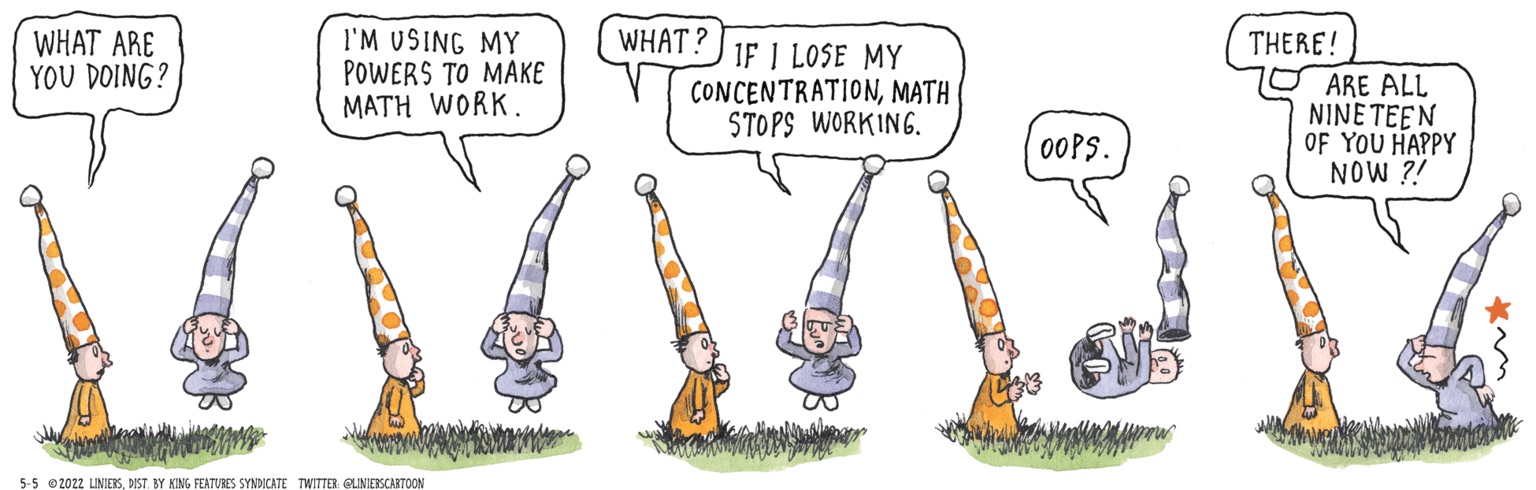
 . It’s equal to zero everywhere, except where
  is zero. When
  or
or  being functions. Many will classify it as a distribution instead. But it is so useful, for a particular kind of problem, that it’s impossible to throw away.
  . And there’s how fast the stick is changing,
  . You can draw these axes; I recommend


 — of milk.
  times.
  . I could be more precise by refilling the mug
  times. I’m also going to suppose that I refill the mug with
 units of milk in the mixture.
  milk in the mixture.
  . And are pretty sure what happens at the fourth and fifth and so on. If you didn’t nod to that, it’s all right. If you’re willing to take me on faith we can continue. If you’re not, that’s good too. Try doing a couple drawings yourself and you may convince yourself. If not, I don’t know. Maybe try, like, getting six white and 24 brown beads, stir them up, take out four at random. Replace all four with brown beads and count, and do that several times over. If you’re short on beads, cut up some paper into squares and write ‘B’ and ‘W’ on each square.
 refills. So my last full mug of tea will have left in it
 of milk. That’s
  as in
as in 
 is the velocity. If we want to emphasize we think of vectors,
  is the position and
  the velocity.
  , or if we want to emphasize its vector nature,
  . Why a name besides the good enough
  , also known as
  . Or, if we’re sure we won’t lose a ‘ mark,
  . Once we are comfortable thinking of how position changes in time we can think of other changes. Velocity’s change in time we call acceleration. This is also a vector, more abstract than position or velocity. Multiply the acceleration by the mass of the thing accelerating and we have a vector called the “force”. That, we at least feel we understand, and can work with.
  , where n is some big enough number like 4.
  . The superscript-T there, “transposition”, lets us use the tools of matrix algebra. This vector describes a point in phase space. Phase space is the collection of all the physically possible positions and velocities for the system.
  , or,
, or,  . This acceleration itself depends on, normally, the positions and velocities. So we can describe this as
  for some function
  . You are surely impressed with this symbol-shuffling. You are less sure why this bother.
  . Or approximate our problem as a matrix problem. This lets us bring in linear algebra tools, and that’s worthwhile.
  . Most of them extend to
  . The result is a classic mathematician’s trick. We can recast a problem as one we have better tools to solve.
  , in the complex conjugate, that element would be
  . Reverse the plus or minus sign of the imaginary component. The shorthand for “the complex conjugate to matrix U” is
  . Also we’ll often just say “the conjugate”, taking the “complex” part as implied.
  .
.  . For a wonder, as matrices go, it doesn’t matter whether you take the transpose or the conjugate first. It’s the same
  . You may ask how people writing this out by hand never mistake
  . This is a good question and I hope to have an answer someday. (I would write it as
  in my notes.)
  .
.  for an identity matrix. If we have to be clear how many rows and columns the matrix has, we write that as a subscript:
  or
or  or
or  or so on.
  is a “diagonal” matrix. A diagonal matrix has zeroes for every element except the diagonal ones. That is, row one, column one; row two, column two; row three, column three; and so on. The elements that trace a path from the upper-left to the lower-right corner of the matrix. (The diagonal from the upper-right to the lower-left we have nothing to do with.) Everything we might do with matrices is easier on a diagonal matrix. So we process our matrix A into this diagonal matrix D. Process it by whatever the heck we’re doing. If we then multiply this by the inverses of U and V? If we calculate
  ? We get whatever our process would have given us had we done it to A. And, since U and V are unitary matrices, it’s easy to find these inverses. Wonderful!
  is a diagonal matrix. And then that’s great. The original H is hard to work with. The diagonalized version? That one we can almost always work with. And then we can go from solutions on the diagonalized version back to solutions on the original. (If the function
  describes the evolution of
  describes the evolution of
  .) The work that U (and
  . I don’t have a good way to describe what this is, physically; we can’t observe it directly. This symmetry, though, manifests as the conservation of electric charge, a thing we rather like.


 is a division algebra.
  is parallelizable, ie, there exist n – 1 tangent vector fields to
  divides
  . There are only three values of ‘n’ that do that. For example.
  . Or you can have an ordered pair,
  . Or an ordered quadruple,
  . Or you can have an ordered octuple,
  . And that’s it. Not that other ordered sets can’t be interesting. They will all diverge far enough from the way real numbers work that you can’t do something that looks like division.
  and know what it meant. We won’t see that for any bigger ordered set of
  outside the stable range”. I know I don’t. I do know when I hear a beautiful string of syllables and that is a joy of mathematics never appreciated enough.


![Comic strip Chaos Butterfly Man: 'Bitten by a radioactive chaos butterfly, Mike Mason gained the powers of a chaos butterfly!' [ Outside a bank ] Mason flaps his arm at an escaping robber. Robber: 'Ha-ha! What harm can THAT do me?' [ Nine days later ] Robber: 'Where did this thunderstorm finally come fr ... YOW!' (He's struck by lightning.)](https://nebusresearch.files.wordpress.com/2020/06/super-fun-pak-comics_ruben-bolling_23-may-2020.gif)
 . Atiyah had started — as an undergraduate — working on projective geometries. This is what one curve looks like projected onto a different surface. This moved

 and that’s your x-coordinate distribution. (This is assuming that we know
  , which equals
  . The
. The  is partial derivatives. The
  is Planck’s constant, a number which in normal systems of measurement is amazingly tiny. And you know how
  . That – symbol is just the minus or the subtraction symbol. So to find the momentum distribution, evaluate
  . This means taking a derivative of the
  in the momentum operator rather than the position operator? Why isn’t one
  and the other
  ? From a mathematical physics perspective, position and momentum are equally good variables. We tend to think of position as fundamental, but that’s surely a result of our happening to be very good at seeing where things are. If we were primarily good at spotting the momentum of things around us, we’d surely see that as the more important variable. When we get into Hamiltonian mechanics we start treating position and momentum as equally fundamental. Even the notation emphasizes how equal they are in importance, and treatment. We stop using ‘x’ or ‘r’ as the variable representing position. We use ‘q’ instead, a mirror to the ‘p’ that’s the standard for momentum. (‘p’ we’ve always used for momentum because … … … uhm. I guess ‘m’ was already committed, for ‘mass’. What I have seen is that it was taken as the first letter in ‘impetus’ with no other work to do. I don’t know that this is true. I’m passing on what I was told explains what looks like an arbitrary choice.)
  and derivatives or worse.
 (roughly 1:1.6), is somehow a uniquely beautiful composition. You may sometimes see memes with some nice-looking animal and various boxes superimposed over it, possibly along with a spiral. The rectangles have the Golden Ratio ratio of width to height. And the ratio is kind of attractive since
  is about 1.618, and
  is about 0.618. It’s a cute pattern,
 proportions, or
  , or even to be particularly consistent about what they like. You might be able to find (say) that the ratio of an eagle’s body length to the wing span is something close to
  . But any real-world thing has a lot of things you can measure. It would be surprising if you couldn’t find something near enough a ratio you liked. The guy is being ridiculous.
![Mathematician: 'Thanks to computer science we no longer need dating. We can produce perfect marriages with simple algorithms.' Assistant: 'ooh!' [ AND SO ] Date-o-Tron, to the mathematician and her assistant: 'There are many women you'd be happier with, but they're already with people whom they prefer to you. Thus, you will be paired with your 4,291th favorite choice. We have a stable equilibrium.' Mathematician: 'Hooray!'](https://nebusresearch.files.wordpress.com/2019/12/saturday-morning-breakfast-cereal_zach-weinersmith_26-november-2019.gif)


 is true. We can suppose that if we cared we could find what function, or functions, f made that equation true. There is shorthand here. A function has a domain, a range, and a rule. The equation part helps us find the rule. The domain and range we get from the problem. Or we take the implicit rule that both are the biggest sets of real-valued numbers for which the rule parses. Sometimes biggest sets of complex-valued numbers. We get so used to saying “the function” to mean “the rule for the function” that we’ll forget to say that’s what we’re doing.

 even has fewer symbols than
  has. But the symbols mean different abstract things. In a quantum mechanics context, ‘A’ and ‘B’ represent — well, possibly matrices. More likely operators. Operators work a lot like functions and I’m going to skip discussing the ways they don’t. Multiplying operators together — B times A, here — works by using the range of one function as the domain of the other. Like, imagine ‘B’ means ‘take the square of’ and ‘A’ means ‘take the sine of’. Then ‘BA’ would mean ‘take the square of the sine of’ (something). The fun part is the ‘AB’ would mean ‘take the sine of the square of’ (something). Which is fun because most of the time, those won’t have the same value. We accept that, mathematically. It turns out to work well for some quantum mechanics properties, even though it doesn’t work like regular arithmetic. So


 or as
or as  and might be used even more often. It turns out
 ![Weenus: 'What's all the noise? I have work in the morning and I'm trying to sleep.' Eight-ball: 'Lettuce [rabbit] just dropped a slice of toast butter-side-up twenty times in a row!' Next panel, they're racing, dragging Lettuce to a flight to Las Vegas.](https://nebusresearch.files.wordpress.com/2019/07/rabbits-against-magic_jonathan-lemon_19-july-2019.gif)


