Do you need to know the formula to tell you what the sum of the first N counting numbers, raised to a power? No, you do not. Not really. It can save a bit of time to know the sum of the numbers raised to the first power. Most mathematicians would know it, or be able to recreate it fast enough:
It’s a neat one. Mariani describes a way to use knowledge of the sum of numbers to the first power to generate a formula for the sum of squares. And then to use the sum of squares formula to generate the sum of cubes. The sum of cubes then lets you get the sub of fourth-powers. And so on. This takes a while to do if you’re interested in the sum of twentieth powers. But do you know how many times you’ll ever need to generate that formula? Anyway, as Mariani notes, this sort of thing is useful if you find yourself at a mathematics competition. Or some other event where you can’t just have the computer calculate this stuff.
Mariani’s process is a great one. Like many mnemonics it doesn’t make literal sense. It expects one to integrate and differentiate polynomials. Anyone likely to be interested in a formula for the sums of twelfth powers knows how to do those in their sleep. But they’re integrating and differentiating polynomials for which, in context, the integrals and derivatives don’t exist. Or at least don’t mean anything. That’s all right. If all you want is the right answer, it’s okay to get there by a wrong method. At least if you verify the answer is right, which the last section of Mariani’s paper does. So, give it a read if you’d like to see a neat mathematical trick to a maybe useful result.
Mr Wu, my Singapore Maths Tuition friend, has offered many fine ideas for A-to-Z topics. This week’s is another of them, and I’m grateful for it.
Ordinary Differential Equations
As a rule, if you can do something with a number, you can do the same thing with a function. Not always, of course, but the exceptions are fewer than you might imagine. I’ll start with one of those things you can do to both.
A powerful thing we learn in (high school) algebra is that we can use a number without knowing what it is. We give it a name like ‘x’ or ‘y’ and describe what we find interesting about it. If we want to know what it is, we (usually) find some equation or set of equations and find what value of x could make that true. If we study enough (college) mathematics we learn its equivalent in functions. We give something a name like f or g or Ψ and describe what we know about it. And then try to find functions which make that true.
There are a couple common types of equation for these not-yet-known functions. The kind you expect to learn as a mathematics major involves differential equations. These are ones where your equation (or equations) involve derivatives of the not-yet-known f. A derivative describes the rate at which something changes. If we imagine the original f is a position, the derivative is velocity. Derivatives can have derivatives also; this second derivative would be the acceleration. And then second derivatives can have derivatives also, and so on, into infinity. When an equation involves a function and its derivatives we have a differential equation.
(The second common type is the integral equation, using a function and its integrals. And a third involves both derivatives and integrals. That’s known as an integro-differential equation, and isn’t life complicated enough? )
Differential equations themselves naturally divide into two kinds, ordinary and partial. They serve different roles. Usually an ordinary differential equation we can describe the change for from knowing only the current situation. (This may include velocities and accelerations and stuff. We could ask what the velocity at an instant means. But never mind that here.) Usually a partial differential equation bases the change where you are on the neighborhood of where your location. If you see holes you can pick in that, you’re right. The precise difference is about the independent variables. If the function f has more than one independent variable, it’s possible to take a partial derivative. This describes how f changes if one variable changes while the others stay fixed. If the function f has only the one independent variable, you can only take ordinary derivatives. So you get an ordinary differential equation.
But let’s speak casually here. If what you’re studying can be fully represented with a dashboard readout? Like, an ordered list of positions and velocities and stuff? You probably have an ordinary differential equation. If you need a picture with a three-dimensional surface or a color map to understand it? You probably have a partial differential equation.
One more metaphor. If you can imagine the thing you’re modeling as a marble rolling around on a hilly table? Odds are that’s an ordinary differential equation. And that representation covers a lot of interesting problems. Marbles on hills, obviously. But also rigid pendulums: we can treat the angle a pendulum makes and the rate at which those change as dimensions of space. The pendulum’s swinging then matches exactly a marble rolling around the right hilly table. Planets in space, too. We need more dimensions — three space dimensions and three velocity dimensions — for each planet. So, like, the Sun-Earth-and-Moon would be rolling around a hilly table with 18 dimensions. That’s all right. We don’t have to draw it. The mathematics works about the same. Just longer.
[ To be precise we need three momentum dimensions for each orbiting body. If they’re not changing mass appreciably, and not moving too near the speed of light, velocity is just momentum times a constant number, so we can use whichever is easier to visualize. ]
We mostly work with ordinary differential equations of either the first or the second order. First order means we have first derivatives in the equation, but never have to deal with more than the original function and its first derivative. Second order means we have second derivatives in the equation, but never have to deal with more than the original function or its first or second derivatives. You’ll never guess what a “third order” differential equation is unless you have experience in reading words. There are some reasons we stick to these low orders like first and second, though. One is that we know of good techniques for solving most first- and second-order ordinary differential equations. For higher-order differential equations we often use techniques that find a related normal old polynomial. Its solution helps with the thing we want. Or we break a high-order differential equation into a set of low-order ones. So yes, again, we search for answers where the light is good. But the good light covers many things we like to look at.
There’s simple harmonic motion, for example. It covers pendulums and springs and perturbations around stable equilibriums and all. This turns out to cover so many problems that, as a physics major, you get a little sick of simple harmonic motion. There’s the Airy function, which started out to describe the rainbow. It turns out to describe particles trapped in a triangular quantum well. The van der Pol equation, about systems where a small oscillation gets energy fed into it while a large oscillation gets energy drained. All kinds of exponential growth and decay problems. Very many functions where pairs of particles interact.
This doesn’t cover everything we would like to do. That’s all right. Ordinary differential equations lend themselves to numerical solutions. It requires considerable study and thought to do these numerical solutions well. But this doesn’t make the subject unapproachable. Few of us could animate the “Pink Elephants on Parade” scene from Dumbo. But could you draw a flip book of two stick figures tossing a ball back and forth? If you’ve had a good rest, a hearty breakfast, and have not listened to the news yet today, so you’re in a good mood?
The flip book ball is a decent example here, too. The animation will look good if the ball moves about the “right” amount between pages. A little faster when it’s first thrown, a bit slower as it reaches the top of its arc, a little faster as it falls back to the catcher. The ordinary differential equation tells us how fast our marble is rolling on this hilly table, and in what direction. So we can calculate how far the marble needs to move, and in what direction, to make the next page in the flip book.
Almost. The rate at which the marble should move will change, in the interval between one flip-book page and the next. The difference, the error, may not be much. But there is a difference between the exact and the numerical solution. Well, there is a difference between a circle and a regular polygon. We have many ways of minimizing and estimating and controlling the error. Doing that is what makes numerical mathematics the high-paid professional industry it is. Our game of catch we can verify by flipping through the book. The motion of four dozen planets and moons attracting one another is harder to be sure we calculate it right.
I said at the top that most anything one can do with numbers one can do with functions also. I would like to close the essay with some great parallel. Like, the way that trying to solve cubic equations made people realize complex numbers were good things to have. I don’t have a good example like that for ordinary differential equations, where the study expanded our ideas of what functions could be. Part of that is that complex numbers are more accessible than the stranger functions. Part of that is that complex numbers have a story behind them. The story features titanic figures like Gerolamo Cardano, Niccolò Tartaglia and Ludovico Ferrari. We see some awesome and weird personalities in 19th century mathematics. But their fights are generally harder to watch from the sidelines and cheer on. And part is that it’s easier to find pop historical treatments of the kinds of numbers. The historiography of what a “function” is is a specialist occupation.
But I can think of a possible case. A tool that’s sometimes used in solving ordinary differential equations is the “Dirac delta function”. Yes, that Paul Dirac. It’s a weird function, written as . It’s equal to zero everywhere, except where is zero. When is zero? It’s … we don’t talk about what it is. Instead we talk about what it can do. The integral of that Dirac delta function times some other function can equal that other function at a single point. It strains credibility to call this a function the way we speak of, like, or being functions. Many will classify it as a distribution instead. But it is so useful, for a particular kind of problem, that it’s impossible to throw away.
So perhaps the parallels between numbers and functions extend that far. Ordinary differential equations can make us notice kinds of functions we would not have seen otherwise.
And with this — I can see the much-postponed end of the Little 2021 Mathematics A-to-Z! You can read all my entries for 2021 at this link, and if you’d like can find all my A-to-Z essays here. How will I finish off the shortest yet most challenging sequence I’ve done yet? Will it be yellow and equivalent to the Axiom of Choice? Answers should come, in a week, if all starts going well.
By the time of 2019 and my sixth A-to-Z series , I had some standard narrative tricks I could deploy. My insistence that everything is polynomials, for example. Anecdotes from my slight academic career. A prose style that emphasizes what we do with the idea of something rather than instructions. That last comes from the idea that if you wanted to know how to compute a Taylor series you’d just look it up on Mathworld or Wikipedia or whatnot. The thing a pop mathematics blog can do is give some reason that you’d want to know how to compute a Taylor series. I regret talking about functions that break Taylor series, though. I have to treat these essays as introducing the idea of a Taylor series to someone who doesn’t know anything about them. And it’s bad form to teach how stuff doesn’t work too close to teaching how it does work. Readers tend to blur what works and what doesn’t together. Still, is a really neat weird function and it’d be a shame to let it go completely unmentioned.
Today’s A To Z term was nominated by APMA, author of the Everybody Makes DATA blog. It was a topic that delighted me to realize I could explain. Then it started to torment me as I realized there is a lot to explain here, and I had to pick something. So here’s where things ended up.
In the mid-2000s I was teaching at a department being closed down. In its last semester I had to teach Computational Quantum Mechanics. The person who’d normally taught it had transferred to another department. But a few last majors wanted the old department’s version of the course, and this pressed me into the role. Teaching a course you don’t really know is a rush. It’s a semester of learning, and trying to think deeply enough that you can convey something to students. This while all the regular demands of the semester eat your time and working energy. And this in the leap of faith that the syllabus you made up, before you truly knew the subject, will be nearly enough right. And that you have not committed to teaching something you do not understand.
So around mid-course I realized I needed to explain finding the wave function for a hydrogen atom with two electrons. The wave function is this probability distribution. You use it to find things like the probability a particle is in a certain area, or has a certain momentum. Things like that. A proton with one electron is as much as I’d ever done, as a physics major. We treat the proton as the center of the universe, immobile, and the electron hovers around that somewhere. Two electrons, though? A thing repelling your electron, and repelled by your electron, and neither of those having fixed positions? What the mathematics of that must look like terrified me. When I couldn’t procrastinate it farther I accepted my doom and read exactly what it was I should do.
It turned out I had known what I needed for nearly twenty years already. Got it in high school.
Of course I’m discussing Taylor Series. The equations were loaded down with symbols, yes. But at its core, the important stuff, was this old and trusted friend.
The premise behind a Taylor Series is even older than that. It’s universal. If you want to do something complicated, try doing the simplest thing that looks at all like it. And then make that a little bit more like you want. And then a bit more. Keep making these little improvements until you’ve got it as right as you truly need. Put that vaguely, the idea describes Taylor series just as well as it describes making a video game or painting a state portrait. We can make it more specific, though.
A series, in this context, means the sum of a sequence of things. This can be finitely many things. It can be infinitely many things. If the sum makes sense, we say the series converges. If the sum doesn’t, we say the series diverges. When we first learn about series, the sequences are all numbers. , for example, which diverges. (It adds to a number bigger than any finite number.) Or , which converges. (It adds to .)
In a Taylor Series, the terms are all polynomials. They’re simple polynomials. Let me call the independent variable ‘x’. Sometimes it’s ‘z’, for the reasons you would expect. (‘x’ usually implies we’re looking at real-valued functions. ‘z’ usually implies we’re looking at complex-valued functions. ‘t’ implies it’s a real-valued function with an independent variable that represents time.) Each of these terms is simple. Each term is the distance between x and a reference point, raised to a whole power, and multiplied by some coefficient. The reference point is the same for every term. What makes this potent is that we use, potentially, many terms. Infinitely many terms, if need be.
Call the reference point ‘a’. Or if you prefer, x0. z0 if you want to work with z’s. You see the pattern. This ‘a’ is the “point of expansion”. The coefficients of each term depend on the original function at the point of expansion. The coefficient for the term that has is the first derivative of f, evaluated at a. The coefficient for the term that has is the second derivative of f, evaluated at a (times a number that’s the same for the squared-term for every Taylor Series). The coefficient for the term that has is the third derivative of f, evaluated at a (times a different number that’s the same for the cubed-term for every Taylor Series).
You’ll never guess what the coefficient for the term with is. Nor will you ever care. The only reason you would wish to is to answer an exam question. The instructor will, in that case, have a function that’s either the sine or the cosine of x. The point of expansion will be 0, , , or .
Otherwise you will trust that this is one of the terms of , ‘n’ representing some counting number too great to be interesting. All the interesting work will be done with the Taylor series either truncated to a couple terms, or continued on to infinitely many.
What a Taylor series offers is the chance to approximate a function we’re genuinely interested in with a polynomial. This is worth doing, usually, because polynomials are easier to work with. They have nice analytic properties. We can automate taking their derivatives and integrals. We can set a computer to calculate their value at some point, if we need that. We might have no idea how to start calculating the logarithm of 1.3. We certainly have an idea how to start calculating . (Yes, it’s 0.3. I’m using a Taylor series with a = 1 as the point of expansion.)
The first couple terms tell us interesting things. Especially if we’re looking at a function that represents something physical. The first two terms tell us where an equilibrium might be. The next term tells us whether an equilibrium is stable or not. If it is stable, it tells us how perturbations, points near the equilibrium, behave.
The first couple terms will describe a line, or a quadratic, or a cubic, some simple function like that. Usually adding more terms will make this Taylor series approximation a better fit to the original. There might be a larger region where the polynomial and the original function are close enough. Or the difference between the polynomial and the original function will be closer together on the same old region.
We would really like that region to eventually grow to the whole domain of the original function. We can’t count on that, though. Roughly, the interval of convergence will stretch from ‘a’ to wherever the first weird thing happens. Weird things are, like, discontinuities. Vertical asymptotes. Anything you don’t like dealing with in the original function, the Taylor series will refuse to deal with. Outside that interval, the Taylor series diverges and we just can’t use it for anything meaningful. Which is almost supernaturally weird of them. The Taylor series uses information about the original function, but it’s all derivatives at a single point. Somehow the derivatives of, say, the logarithm of x around x = 1 give a hint that the logarithm of 0 is undefinable. And so they won’t help us calculate the logarithm of 3.
Things can be weirder. There are functions that just break Taylor series altogether. Some are obvious. A function needs lots of derivatives at a point to have a good Taylor series approximation. So, many fractal curves won’t have a Taylor series approximation. These curves are all corners, points where they aren’t continuous or where derivatives don’t exist. Some are obviously designed to break Taylor series approximations. We can make a function that follows different rules if x is rational than if x is irrational. There’s no approximating that, and you’d blame the person who made such a function, not the Taylor series. It can be subtle. The function defined by the rule , with the note that if x is zero then f(x) is 0, seems to satisfy everything we’d look for. It’s a function that’s mostly near 1, that drops down to being near zero around where x = 0. But its Taylor series expansion around a = 0 is a horizontal line always at 0. The interval of convergence can be a single point, challenging our idea of what an interval is.
That’s all right. If we can trust that we’re avoiding weird parts, Taylor series give us an outstanding new tool. Grant that the Taylor series describes a function with the same rule as our original function. The Taylor series is often easier to work with, especially if we’re working on differential equations. We can automate, or at least find formulas for, taking the derivative of a polynomial. Or adding together derivatives of polynomials. Often we can attack a differential equation too hard to solve otherwise by supposing the answer is a polynomial. This is essentially what that quantum mechanics problem used, and why the tool was so familiar when I was in a strange land.
Roughly. What I was actually doing was treating the function I wanted as a power series. This is, like the Taylor series, the sum of a sequence of terms, all of which are times some coefficient. What makes it not a Taylor series is that the coefficients weren’t the derivatives of any function I knew to start. But the experience of Taylor series trained me to look at functions as things which could be approximated by polynomials.
This gives us the hint to look at other series that approximate interesting functions. We get a host of these, with names like Laurent series and Fourier series and Chebyshev series and such. Laurent series look like Taylor series but we allow powers to be negative integers as well as positive ones. Fourier series do away with polynomials. They instead use trigonometric functions, sines and cosines. Chebyshev series build on polynomials, but not on pure powers. They’ll use orthogonal polynomials. These behave like perpendicular directions do. That orthogonality makes many numerical techniques behave better.
The Taylor series is a great introduction to these tools. Its first several terms have good physical interpretations. Its calculation requires tools we learn early on in calculus. The habits of thought it teaches guides us even in unfamiliar territory.
And I feel very relieved to be done with this. I often have a few false starts to an essay, but those are mostly before I commit words to text editor. This one had about four branches that now sit in my scrap file. I’m glad to have a deadline forcing me to just publish already.
This week’s topic is one of several suggested again by Mr Wu, blogger and Singaporean mathematics tutor. He’d suggested several topics, overlapping in their subject matter, and I was challenged to pick one.
Monte Carlo.
The reputation of mathematics has two aspects: difficulty and truth. Put “difficulty” to the side. “Truth” seems inarguable. We expect mathematics to produce sound, deductive arguments for everything. And that is an ideal. But we often want to know things we can’t do, or can’t do exactly. We can handle that often. If we can show that a number we want must be within some error range of a number we can calculate, we have a “numerical solution”. If we can show that a number we want must be within every error range of a number we can calculate, we have an “analytic solution”.
There are many things we’d like to calculate and can’t exactly. Many of them are integrals, which seem like they should be easy. We can represent any integral as finding the area, or volume, of a shape. The trick is that there’s only a few shapes with volumes we can find exact formulas for. You may remember the area of a triangle or a parallelogram. You have no idea what the area of a regular nonagon is. The trick we rely on is to approximate the shape we want with shapes we know formulas for. This usually gives us a numerical solution.
If you’re any bit devious you’ve had the impulse to think of a shape that can’t be broken up like that. There are such things, and a good swath of mathematics in the late 19th and early 20th centuries was arguments about how to handle them. I don’t mean to discuss them here. I’m more interested in the practical problems of breaking complicated shapes up into simpler ones and adding them all together.
One catch, an obvious one, is that if the shape is complicated you need a lot of simpler shapes added together to get a decent approximation. Less obvious is that you need way more shapes to do a three-dimensional volume well than you need for a two-dimensional area. That’s important because you need even way-er more to do a four-dimensional hypervolume. And more and more and more for a five-dimensional hypervolume. And so on.
That matters because many of the integrals we’d like to work out represent things like the energy of a large number of gas particles. Each of those particles carries six dimensions with it. Three dimensions describe its position and three dimensions describe its momentum. Worse, each particle has its own set of six dimensions. The position of particle 1 tells you nothing about the position of particle 2. So you end up needing ridiculously,impossibly many shapes to get even a rough approximation.
With no alternative, then, we try wisdom instead. We train ourselves to think of deductive reasoning as the only path to certainty. By the rules of deductive logic it is. But there are other unshakeable truths. One of them is randomness.
We can show — by deductive logic, so we trust the conclusion — that the purely random is predictable. Not in the way that lets us say how a ball will bounce off the floor. In the way that we can describe the shape of a great number of grains of sand dropped slowly on the floor.
The trick is one we might get if we were bad at darts. If we toss darts at a dartboard, badly, some will land on the board and some on the wall behind. How many hit the dartboard, compared to the total number we throw? If we’re as likely to hit every spot of the wall, then the fraction that hit the dartboard, times the area of the wall, should be about the area of the dartboard.
So we can do something equivalent to this dart-throwing to find the volumes of these complicated, hyper-dimensional shapes. It’s a kind of numerical integration. It isn’t particularly sensitive to how complicated the shape is, though. It takes more work to find the volume of a shape with more dimensions, yes. But it takes less more-work than the breaking-up-into-known-shapes method does. There are wide swaths of mathematics and mathematical physics where this is the best way to calculate the integral.
This bit that I’ve described is called “Monte Carlo integration”. The “integration” part of the name because that’s what we started out doing. To call it “Monte Carlo” implies either the method was first developed there or the person naming it was thinking of the famous casinos. The case is the latter. Monte Carlo methods as we know them come from Stanislaw Ulam, mathematical physicist working on atomic weapon design. While ill, he got to playing the game of Canfield solitaire, about which I know nothing except that Stanislaw Ulam was playing it in 1946 while ill. He wondered what the chance was that a given game was winnable. The most practical approach was sampling: set a computer to play a great many games and see what fractions of them were won. (The method comes from Ulam and John von Neumann. The name itself comes from their colleague Nicholas Metropolis.)
There are many Monte Carlo methods, with integration being only one very useful one. They hold in common that they’re build on randomness. We try calculations — often simple ones — many times over with many different possible values. And the regularity, the predictability, of randomness serves us. The results come together to an average that is close to the thing we do want to know.
Mental arithmetic is fun. It has some use, yes. It’s always nice when you’re doing work to have some idea what a reasonable answer looks like. But mostly it’s fun to be able to spot, oh, 24 times 16, that’s got to be a little under 400.
I ran across this post, by Math1089, with a neat trick for certain multiplications. It’s limited in scope. Most mental-arithmetic tricks are; they have certain problems they do well and you need to remember a grab bag that covers enough to be useful. Here, the case is multiplying two numbers that start the same way, and whose ends are complements. That is, the ends add together to 10. (Or, to 100, or 1000, or some other power of two.) So, for example, you could use this trick to multiply together 41 and 49, or 64 and 66. (Or, if you needed, to multiply 2038 by 2062.)
It won’t directly solve 41 times 39, though, nor 64 times 65. But you can hack it together. 64 times 65 is 64 times 66 — you have a trick for that — minus 64. 41 times 39 is tougher, but, it’s 41 times 49 minus 41 times 10. 41 times 10 is easy to do. This is what I mean by learning a grab bag of tricks. You won’t outpace someone who has their calculator out and ready to go. But you might outpace someone who has to get their calculator out, and you’ll certainly impress them.
So it’s clever, and not hard to learn. If you feel like testing your high-school algebra prowess you can even work out why this trick works, and why it has the limits it does.
The talk of the catenary and the brachistochrone give away that this is a calculus paper. The catenary and the brachistochrone are some of the oldest problems in calculus as we know it. The catenary is the problem of what shape a weighted chain takes under gravity. The brachistochrone is the problem of what path a beam of light traces out moving through regions with different indexes of refraction. (As in, through films of glass or water or such.) Straight lines and circles we’ve heard of from other places.
The paper relies on calculus so if you’re not comfortable with that, well, skim over the lines with symbols. Rojas discusses the ways that we can treat all these different shapes as solutions of related, very similar problems. And there’s some talk about calculating approximate solutions. There is special delight in this as these are problems that can be done by an analog computer. You can build a tool to do some of these calculations. And I do mean “you”; the approach is to build a box, like, the sort of thing you can do by cutting up plastic sheets and gluing them together and setting toothpicks or wires on them. Then dip the model into a soap solution. Lift it out slowly and take a good picture of the soapy surface.
This is not as quick, or as precise, as fiddling with a Matlab or Octave or Mathematica simulation. But it can be much more fun.
I don’t yet have actual words committed to text editor for this year’s little A-to-Z yet. Soon, though. Rather than leave things completely silent around here, I’d like to re-share an old sequence about something which delighted me. A lon while ago I read Edmund Callis Berkeley’s Giant Brains: Or Machines That Think. It’s a book from 1949 about numerical computing. And it explained just how to really calculate logarithms.
Anyone who knows calculus knows, in principle, how to calculate a logarithm. I mean as in how to get a numerical approximation to whatever the log of 25 is. If you didn’t have a calculator that did logarithms, but you could reliably multiply and add numbers? There’s a polynomial, one of a class known as Taylor Series, that — if you add together infinitely many terms — gives the exact value of a logarithm. If you only add a finite number of terms together, you get an approximation.
That suffices, in principle. In practice, you might have to calculate so many terms and add so many things together you forget why you cared what the log of 25 was. What you want is how to calculate them swiftly. Ideally, with as few calculations as possible. So here’s a set of articles I wrote, based on Berkeley’s book, about how to do that.
Machines That Give You Logarithms explains how to use those tools. And lays out how to get the base-ten logarithm for most numbers that you would like with a tiny bit of computing work. I showed off an example of getting the logarithm of 47.2286 using only three divisions, four additions, and a little bit of looking up stuff.
Without Machines That Think About Logarithms closes it out. One catch with the algorithm described is that you need to work out some logarithms ahead of time and have them on hand, ready to look up. They’re not ones that you care about particularly for any problem, but they make it easier to find the logarithm you do want. This essay talks about which logarithms to calculate, in order to get the most accurate results for the logarithm you want, using the least custom work possible.
And that’s the series! With that, in principle, you have a good foundation in case you need to reinvent numerical computing.
I am made aware that a section of Twitter argues about how to evaluate an expression. There may be more than one of these going around, but the expression I’ve seen is:
Many people feel that the challenge is knowing the order of operations. This is reasonable. That is, that to evaluate arithmetic, you evaluate terms inside parentheses first. Then terms within exponentials. Then multiplication and division. Then addition and subtraction. This is often abbreviated as PEMDAS, and made into a mnemonic like “Please Excuse My Dear Aunt Sally”.
That is fine as far as it goes. Many people likely start by adding the 1 and 2 within the parentheses, and that’s fair. Then they get:
Putting two quantities next to one another, as the 2 and the (3) are, means to multiply them. And then comes the disagreement: does this mean take and multiply that by 3, in which case the answer is 9? Or does it mean take 6 divided by , in which case the answer is 1?
And there is the trick. Depending on which way you choose to parse these instructions you get different answers. But you don’t get to do that, not and have arithmetic. So the answer is that this expression has no answer. The phrasing is ambiguous and can’t be resolved.
I’m aware there are people who reject this answer. They picked up along the line somewhere a rule like “do multiplication and division from left to right”. And a similar rule for addition and subtraction. This is wrong, but understandable. The left-to-right “rule” is a decent heuristic, a guide to how to attack a problem too big to do at once. The rule works because multiplication-and-division associates. The quantity a-times-b, multiplied by c, has to be the same number as the quantity a multiplied by the quantity b-times-c. The rule also works for addition-and-subtraction because addition associates too. The quantity a-plus-b, plus the quantity c, has to be the same as the quantity a plus the quantity b-plus-c.
This left-to-right “rule”, though, just helps you evaluate a meaningful expression. It would be just as valid to do all the multiplications-and-divisions from right-to-left. If you get different values working left-to-right from right-to-left, you have a meaningless expression.
But you also start to see why mathematicians tend to avoid the symbol. We understand, for example, to mean . Carry that out and then there’s no ambiguity about
I understand the desire to fix an ambiguity. Believe me. I’m a know-it-all; I only like ambiguities that enable logic-based jokes. (“Would you like ice cream or cake?” “Yes.”) But the rules that could remove the ambiguity in also remove associativity from multiplication. Once you do that, you’re not doing arithmetic anymore. Resist the urge.
(And the mnemonic is a bit dangerous. We can say division has the same priority as multiplication, but we also say “multiplication” first. I bet you can construct an ambiguous expression which would mislead someone who learned Please Excuse Dear Miss Sally Andrews.)
And now a qualifier: computer languages will often impose doing a calculation in some order. Usually left-to-right. The microchips doing the work need to have some instructions. Spotting all possible ambiguous phrasings ahead of time is a challenge. But we accept our computers doing not-quite-actual-arithmetic. They’re able to do not-quite-actual-arithmetic much faster and more reliably than we can. This makes the compromise worthwhile. We need to remember the difference between what the computer does and the calculation we intend.
And another qualifier: it is possible to do interesting mathematics with operations that aren’t associative. But if you are it’s in your research as a person with a postgraduate degree in mathematics. It’s possible it might fit in social media, but I would be surprised. It won’t draw great public attention, anyway.
I intend to post something inspired by the comics. I’m not ready just yet. Until then, though, I’d like to share a neat article published in Nature. It’s about paper.
The skeptical reader might say this is obvious. They’re invited to write a simulation that takes a set of fold lines and predicts which sides of the paper are angled out and which are angled in. The skeptical reader may also ask who cares about paper. It’s paper because many mathematics problems start from the kinds of things one sets one’s hands on. Anyone who’s seen a crack growing across their sidewalk, though — or across their countertop, or their grandfather’s desk — realizes there are things we don’t understand about how things break. And why they break that way. And, more generally, there’s a lot we don’t understand about how complicated “natural” shapes form. The big interest in this is how long molecules crumple up. The shapes of these govern how they behave, and it’d be nice to understand that more.
Rosenbluth was a PhD in physics (and an Olympics-qualified fencer). Her postdoctoral work was with the Atomic Energy Commission, bringing her to a position at Los Alamos National Laboratory in the early 1950s. And a moment in computer science that touches very many people’s work, my own included. This is in what we call Metropolis-Hastings Markov Chain Monte Carlo.
Monte Carlo methods are numerical techniques that rely on randomness. The name references the casinos. Markov Chain refers to techniques that create a sequence of things. Each thing exists in some set of possibilities. If we’re talking about Markov Chain Monte Carlo this is usually an enormous set of possibilities, too many to deal with by hand, except for little tutorial problems. The trick is that what the next item in the sequence is depends on what the current item is, and nothing more. This may sound implausible — when does anything in the real world not depend on its history? — but the technique works well regardless. Metropolis-Hastings is a way of finding states that meet some condition well. Usually this is a maximum, or minimum, of some interesting property. The Metropolis-Hastings rule has the chance of going to an improved state, one with more of whatever the property we like, be 1, a certainty. The chance of going to a worsened state, with less of the property, be not zero. The worse the new state is, the less likely it is, but it’s never zero. The result is a sequence of states which, most of the time, improve whatever it is you’re looking for. It sometimes tries out some worse fits, in the hopes that this leads us to a better fit, for the same reason sometimes you have to go downhill to reach a larger hill. The technique works quite well at finding approximately-optimum states when it’s hard to find the best state, but it’s easy to judge which of two states is better. Also when you can have a computer do a lot of calculations, because it needs a lot of calculations.
So here we come to Rosenbluth. She and her then-husband, according to an interview he gave in 2003, were the primary workers behind the 1953 paper that set out the technique. And, particularly, she wrote the MANIAC computer program which ran the algorithm. It’s important work and an uncounted number of mathematicians, physicists, chemists, biologists, economists, and other planners have followed. She would go on to study statistical mechanics problems, in particular simulations of molecules. It’s still a rich field of study.
This is easy. The velocity is the first derivative of the position. First derivative with respect to time, if you must know. That hardly needed an extra week to write.
Yes, there’s more. There is always more. Velocity is important by itself. It’s also important for guiding us into new ideas. There are many. One idea is that it’s often the first good example of vectors. Many things can be vectors, as mathematicians see them. But the ones we think of most often are “some magnitude, in some direction”.
The position of things, in space, we describe with vectors. But somehow velocity, the changes of positions, seems more significant. I suspect we often find static things below our interest. I remember as a physics major that my Intro to Mechanics instructor skipped Statics altogether. There are many important things, like bridges and roofs and roller coaster supports, that we find interesting because they don’t move. But the real Intro to Mechanics is stuff in motion. Balls rolling down inclined planes. Pendulums. Blocks on springs. Also planets. (And bridges and roofs and roller coaster supports wouldn’t work if they didn’t move a bit. It’s not much though.)
So velocity shows us vectors. Anything could, in principle, be moving in any direction, with any speed. We can imagine a thing in motion inside a room that’s in motion, its net velocity being the sum of two vectors.
And they show us derivatives. A compelling answer to “what does differentiation mean?” is “it’s the rate at which something changes”. Properly, we can take the derivative of any quantity with respect to any variable. But there are some that make sense to do, and position with respect to time is one. Anyone who’s tried to catch a ball understands the interest in knowing.
We take derivatives with respect to time so often we have shorthands for it, by putting a ‘ mark after, or a dot above, the variable. So if x is the position (and it often is), then is the velocity. If we want to emphasize we think of vectors, is the position and the velocity.
Velocity has another common shorthand. This is , or if we want to emphasize its vector nature, . Why a name besides the good enough ? It helps us avoid misplacing a ‘ mark in our work, for one. And giving velocity a separate symbol encourages us to think of the velocity as independent from the position. It’s not — not exactly — independent. But knowing that a thing is in the lawn outside tells us nothing about how it’s moving. Velocity affects position, in a process so familiar we rarely consider how there’s parts we don’t understand about it. But velocity is also somehow also free of the position at an instant.
Velocity also guides us into a first understanding of how to take derivatives. Thinking of the change in position over smaller and smaller time intervals gets us to the “instantaneous” velocity by doing only things we can imagine doing with a ruler and a stopwatch.
Velocity has a velocity. , also known as . Or, if we’re sure we won’t lose a ‘ mark, . Once we are comfortable thinking of how position changes in time we can think of other changes. Velocity’s change in time we call acceleration. This is also a vector, more abstract than position or velocity. Multiply the acceleration by the mass of the thing accelerating and we have a vector called the “force”. That, we at least feel we understand, and can work with.
Acceleration has a velocity too, a rate of change in time. It’s called the “jerk” by people telling you the change in acceleration in time is called the “jerk”. (I don’t see the term used in the wild, but admit my experience is limited.) And so on. We could, in principle, keep taking derivatives of the position and keep finding new changes. But most physics problems we find interesting use just a couple of derivatives of the position. We can label them, if we need, , where n is some big enough number like 4.
We can bundle them in interesting ways, though. Come back to that mention of treating position and velocity of something as though they were independent coordinates. It’s a useful perspective. Imagine the rules about how particles interacting with one another and with their environment. These usually have explicit roles for position and velocity. (Granting this may reflect a selection bias. But these do cover enough interesting problems to fill a career.)
So we create a new vector. It’s made of the positition and the velocity. We’d write it out as . The superscript-T there, “transposition”, lets us use the tools of matrix algebra. This vector describes a point in phase space. Phase space is the collection of all the physically possible positions and velocities for the system.
What’s the derivative, in time, of this point in phase space? Glad to say we can do this piece by piece. The derivative of a vector is the derivative of each component of a vector. So the derivative of is , or, . This acceleration itself depends on, normally, the positions and velocities. So we can describe this as for some function . You are surely impressed with this symbol-shuffling. You are less sure why this bother.
The bother is a trick of ordinary differential equations. All differential equations are about how a function-to-be-determined and its derivatives relate to one another. In ordinary differential equations, the function-to-be-determined depends on a single variable. Usually it’s called x or t. There may be many derivatives of f. This symbol-shuffling rewriting takes away those higher-order derivatives. We rewrite the equation as a vector equation of just one order. There’s some point in phase space, and we know what its velocity is. That we do because in this form many problems can be written as a matrix problem: . Or approximate our problem as a matrix problem. This lets us bring in linear algebra tools, and that’s worthwhile.
It also lets us bring in numerical tools. Numerical mathematics has developed many methods to solve the ordinary differential equation. Most of them extend to . The result is a classic mathematician’s trick. We can recast a problem as one we have better tools to solve.
It calls on a more abstract idea of what a “velocity” might be. We can explain what the thing that’s “moving” and what it’s moving through are, given time. But the instincts we develop from watching ordinary things move help us in these new territories. This is also a classic mathematician’s trick. It may seem like all mathematicians do is develop tricks to extend what they already do. I can’t say this is wrong.
Mr Wu, author of the Singapore Maths Tuition blog, asked me to explain a technical term today. I thought that would be a fun, quick essay. I don’t learn very fast, do I?
A note on style. I make reference here to “Big-O” and “Little-O”, capitalizing and hyphenating them. This is to give them visual presence as a name. In casual discussion they’re just read, or said, as the two words or word-and-a-letter. Often the Big- or Little- gets dropped and we just talk about O. An O, without further context, in my experience means Big-O.
The part of me that wants smooth consistency in prose urges me to write “Little-o”, as the thing described is represented with a lowercase ‘o’. But Little-o sounds like a midway game or an Eyerly Aircraft Company amusement park ride. And I never achieve consistency in my prose anyway. Maybe for the book publication. Until I’m convinced another is better, though, “Little-O” it is.
When I first went to college I had a campus post office box. I knew my box number. I also knew the length of the sluggish line for the combination lock code. The lock was a dial, lettered A through J. Being a young STEM-class idiot I thought, boy, would it actually be quicker to pick the lock than wait for the line? A three-letter combination, of ten options? That’s 1,000 possibilities. If I could try five a minute that’s, at worst, three hours 20 minutes. Combination might be anywhere in that set; I might get lucky. I could expect to spend 80 minutes picking my lock.
I decided to wait in line instead, and good that I did. I was unaware lock settings might not be a letter, like ‘A’. It could be the midway point between adjacent letters, like ‘AB’. That meant there were eight times as many combinations as I estimated, and I could expect to spend over ten hours. Even the slow line was faster than that. It transpired that my combination had two of these midway letters.
But that’s a little demonstration of algorithmic complexity. Also in cracking passwords by trial-and-error. Doubling the set of possible combination codes octuples the time it takes to break into the set. Making the combination longer would also work; each extra letter would multiply the cracking time by twenty. So you understand why your password should include “special characters” like punctuation, but most of all should be long.
We’re often interested in how long to expect a task to take. Sometimes we’re interested in the typical time it takes. Often we’re interested in the longest it could ever take. If we have a deterministic algorithm, we can say. We can count how many steps it takes. Sometimes this is easy. If we want to add two two-digit numbers together we know: it will be, at most, three single-digit additions plus, maybe, writing down a carry. (To add 98 and 37 is adding 8 + 7 to get 15, to add 9 + 3 to get 12, and to take the carry from the 15, so, 1 + 12 to get 13, so we have 135.) We can get a good quarrel going about what “a single step” is. We can argue whether that carry into the hundreds column is really one more addition. But we can agree that there is some smallest bit of arithmetic work, and proceed from that.
For any algorithm we have something that describes how big a thing we’re working on. It’s often ‘n’. If we need more than one variable to describe how big it is, ‘m’ gets called up next. If we’re estimating how long it takes to work on a number, ‘n’ is the number of digits in the number. If we’re thinking about a square matrix, ‘n’ is the number of rows and columns. If it’s a not-square matrix, then ‘n’ is the number of rows and ‘m’ the number of columns. Or vice-versa; it’s your matrix. If we’re looking for an item in a list, ‘n’ is the number of items in the list. If we’re looking to evaluate a polynomial, ‘n’ is the order of the polynomial.
In normal circumstances we don’t work out how many steps some operation does take. It’s more useful to know that multiplying these two long numbers would take about 900 steps than that it would need only 816. And so this gives us an asymptotic estimate. We get an estimate of how much longer cracking the combination lock will take if there’s more letters to pick from. This allowing that some poor soul will get the combination A-B-C.
There are a couple ways to describe how long this will take. The more common is the Big-O. This is just the letter, like you find between N and P. Since that’s easy, many have taken to using a fancy, vaguely cursive O, one that looks like . I agree it looks nice. Particularly, though, we write , where f is some function. In practice, we’ll see functions like or or . Usually something simple like that. It can be tricky. There’s a scheme for multiplying large numbers together that’s . What you will not see is something like , or or such. This comes to what we mean by the Big-O.
It’ll be convenient for me to have a name for the actual number of steps the algorithm takes. Let me call the function describing that g(n). Then g(n) is if once n gets big enough, g(n) is always less than C times f(n). Here c is some constant number. Could be 1. Could be 1,000,000. Could be 0.00001. Doesn’t matter; it’s some positive number.
There’s some neat tricks to play here. For example, the function ‘‘ is . It’s also and and . The function ‘‘ is also and those later terms, but it is not . And you can see why is right out.
There is also a Little-O notation. It, too, is an upper bound on the function. But it is a stricter bound, setting tighter restrictions on what g(n) is like. You ask how it is the stricter bound gets the minuscule letter. That is a fine question. I think it’s a quirk of history. Both symbols come to us through number theory. Big-O was developed first, published in 1894 by Paul Bachmann. Little-O was published in 1909 by Edmund Landau. Yes, the one with the short Hilbert-like list of number theory problems. In 1914 G H Hardy and John Edensor Littlewood would work on another measure and they used Ω to express it. (If you see the letter used for Big-O and Little-O as the Greek omicron, then you see why a related concept got called omega.)
What makes the Little-O measure different is its sternness. g(n) is if, for every positive number C, whenever n is large enough g(n) is less than or equal to C times f(n). I know that sounds almost the same. Here’s why it’s not.
If g(n) is , then you can go ahead and pick a C and find that, eventually, . If g(n) is , then I, trying to sabotage you, can go ahead and pick a C, trying my best to spoil your bounds. But I will fail. Even if I pick, like a C of one millionth of a billionth of a trillionth, eventually f(n) will be so big that . I can’t find a C small enough that f(n) doesn’t eventually outgrow it, and outgrow g(n).
This implies some odd-looking stuff. Like, that the function n is not . But the function n is at least , and and those other fun variations. Being Little-O compels you to be Big-O. Big-O is not compelled to be Little-O, although it can happen.
These definitions, for Big-O and Little-O, I’ve laid out from algorithmic complexity. It’s implicitly about functions defined on the counting numbers. But there’s no reason I have to limit the ideas to that. I could define similar ideas for a function g(x), with domain the real numbers, and come up with an idea of being on the order of f(x).
We make some adjustments to this. The important one is that, with algorithmic complexity, we assumed g(n) had to be a positive number. What would it even mean for something to take minus four steps to complete? But a regular old function might be zero or negative or change between negative and positive. So we look at the absolute value of g(x). Is there some value of C so that, when x is big enough, the absolute value of g(x) stays less than C times f(x)? If it does, then g(x) is . Is it the case that for every positive number C it’s true that g(x) is less than C times f(x), once x is big enough? Then g(x) is .
Fine, but why bother defining this?
A compelling answer is that it gives us a way to describe how different a function is from an approximation to that function. We are always looking for approximations to functions because most functions are hard. We have a small set of functions we like to work with. Polynomials are great numerically. Exponentials and trig functions are great analytically. That’s about all the functions that are easy to work with. Big-O notation particularly lets us estimate how bad an error we make using the approximation.
For example, the Runge-Kutta method numerically approximates solutions to ordinary differential equations. It does this by taking the information we have about the function at some point x to approximate its value at a point x + h. ‘h’ is some number. The difference between the actual answer and the Runge-Kutta approximation is . We use this knowledge to make sure our error is tolerable. Also, we don’t usually care what the function is at x + h. It’s just what we can calculate. What we want is the function at some point a fair bit away from x, call it x + L. So we use our approximate knowledge of conditions at x + h to approximate the function at x + 2h. And use x + 2h to tell us about x + 3h, and from that x + 4h and so on, until we get to x + L. We’d like to have as few of these uninteresting intermediate points as we can, so look for as big an h as is safe.
That context may be the more common one. We see it, particularly, in Taylor Series and other polynomial approximations. For example, the sine of a number is approximately:
This has consequences. It tells us, for example, that if x is about 0.1, this approximation is probably pretty good. So it is: the sine of 0.1 (radians) is about 0.0998334166468282 and that’s exactly what five terms here gives us. But it also warns that if x is about 10, this approximation may be gibberish. And so it is: the sine of 10.0 is about -0.5440 and the polynomial is about 1448.27.
The connotation in using Big-O notation here is that we look for small h’s, and for to be a tiny number. It seems odd to use the same notation with a large independent variable and with a small one. The concept carries over, though, and helps us talk efficiently about this different problem.
Today’s topic suggestion was suggested by bunnydoe. I know of a project bunnydoe runs, but not whether it should be publicized. It is another biographical piece. Biographies and complex numbers, that seems to be the theme of this year.
The exact suggestion I got for L was “Leibniz, the inventor of Calculus”. I can’t in good conscience offer that. This isn’t to deny Leibniz’s critical role in calculus. We rely on many of the ideas he’d had for it. We especially use his notation. But there are few great big ideas that can be truly credited to an inventor, or even a team of inventors. Put aside the sorry and embarrassing priority dispute with Isaac Newton. Many mathematicians in the 16th and 17th century were working on how to improve the Archimedean “method of exhaustion”. This would find the areas inside select curves, integral calculus. Johannes Kepler worked out the areas of ellipse slices, albeit with considerable luck. Gilles Roberval tried working out the area inside a curve as the area of infinitely many narrow rectangular strips. We still learn integration from this. Pierre de Fermat recognized how tangents to a curve could find maximums and minimums of functions. This is a critical piece of differential calculus. Isaac Barrow, Evangelista Torricelli (of barometer fame), Pietro Mengoli, and Stephano Angeli all pushed mathematics towards calculus. James Gregory proved, in geometric form, the relationship between differentiation and integration. That relationship is the Fundamental Theorem of Calculus.
This is not to denigrate Leibniz. We don’t dismiss the Wright Brothers though we know that without them, Alberto Santos-Dumont or Glenn Curtiss or Samuel Langley would have built a workable airplane anyway. We have Leibniz’s note, dated the 29th of October, 1675 (says Florian Cajori), writing out to mean the sum of all l’s. By mid-November he was integrating functions, and writing out his work as . Any mathematics or physics or chemistry or engineering major today would recognize that. A year later he was writing things like , which we’d also understand if not quite care to put that way.
Though we use his notation and his basic tools we don’t exactly use Leibniz’s particular ideas of what calculus means. It’s been over three centuries since he published. It would be remarkable if he had gotten the concepts exactly and in the best of all possible forms. Much of Leibniz’s calculus builds on the idea of a differential. This is a quantity that’s smaller than any positive number but also larger than zero. How does that make sense? George Berkeley argued it made not a lick of sense. Mathematicians frowned, but conceded Berkeley was right. By the mid-19th century they had a rationale for differentials that avoided this weird sort of number.
It’s hard to avoid the differential’s lure. The intuitive appeal of “imagine moving this thing a tiny bit” is always there. In science or engineering applications it’s almost mandatory. Few things we encounter in the real world have the kinds of discontinuity that create logic problems for differentials. Even in pure mathematics, we will look at a differential equation like and rewrite it as . Leibniz’s notation gives us the idea that taking derivatives is some kind of fraction. It isn’t, but in many problems we act as though it were. It works out often enough we forget that it might not.
Better, though. From the 1960s Abraham Robinson and others worked out a different idea of what real numbers are. In that, differentials have a rigorous logical definition. We call the mathematics which uses this “non-standard analysis”. The name tells something of its use. This is not to call it wrong. It’s merely not what we learn first, or necessarily at all. And it is Leibniz’s differentials. 304 years after his death there is still a lot of mathematics he could plausibly recognize.
There is still a lot of still-vital mathematics that he touched directly. Leibniz appears to be the first person to use the term “function”, for example, to describe that thing we’re plotting with a curve. He worked on systems of linear equations, and methods to find solutions if they exist. This technique is now called Gaussian elimination. We see the bundling of the equations’ coefficients he did as building a matrix and finding its determinant. We know that technique, today, as Cramer’s Rule, after Gabriel Cramer. The Japanese mathematician Seki Takakazu had discovered determinants before Leibniz, though.
Leibniz tried to study a thing he called “analysis situs”, which two centuries on would be a name for topology. My reading tells me you can get a good fight going among mathematics historians by asking whether he was a pioneer in topology. So I’ll decline to take a side in that.
In the 1680s he tried to create an algebra of thought, to turn reasoning into something like arithmetic. His goal was good: we see these ideas today as Boolean algebra, and concepts like conjunction and disjunction and negation and the empty set. Anyone studying logic knows these today. He’d also worked in something we can see as symbolic logic. Unfortunately for his reputation, the papers he wrote about that went unpublished until late in the 19th century. By then other mathematicians, like Gottlob Frege and Charles Sanders Peirce, had independently published the same ideas.
We give Leibniz’ name to a particular series that tells us the value of π:
(The Indian mathematician Madhava of Sangamagrama knew the formula this comes from by the 14th century. I don’t know whether Western Europe had gotten the news by the 17th century. I suspect it hadn’t.)
The drawback to using this to figure out digits of π is that it takes forever to use. Taking ten decimal digits of π demands evaluating about five billion terms. That’s not hyperbole; it just takes like forever to get its work done.
Which is something of a theme in Leibniz’s biography. He had a great many projects. Some of them even reached a conclusion. Many did not, and instead sprawled out with great ambition and sometimes insight before getting lost. Consider a practical one: he believed that the use of wind-driven propellers and water pumps could drain flooded mines. (Mines are always flooding.) In principle, he was right. But they all failed. Leibniz blamed deliberate obstruction by administrators and technicians. He even blamed workers afraid that new technologies would replace their jobs. Yet even in this failure he observed and had bracing new thoughts. The geology he learned in the mines project made him hypothesize that the Earth had been molten. I do not know the history of geology well enough to say whether this was significant to that field. It may have been another frustrating moment of insight (lucky or otherwise) ahead of its time but not connected to the mainstream of thought.
Another project, tantalizing yet incomplete: the “stepped reckoner”, a mechanical arithmetic machine. The design was to do addition and subtraction, multiplication and division. It’s a breathtaking idea. It earned him election into the (British) Royal Society in 1673. But it never was quite complete, never getting carries to work fully automatically. He never did finish it, and lost friends with the Royal Society when he moved on to other projects. He had a note describing a machine that could do some algebraic operations. In the 1690s he had some designs for a machine that might, in theory, integrate differential equations. It’s a fantastic idea. At some point he also devised a cipher machine. I do not know if this is one that was ever used in its time.
His greatest and longest-lasting unfinished project was for his employer, the House of Brunswick. Three successive Brunswick rulers were content to let Leibniz work on his many side projects. The one that Ernest Augustus wanted was a history of the Guelf family, in the House of Brunswick. One that went back to the time of Charlemagne or earlier if possible. The goal was to burnish the reputation of the house, which had just become a hereditary Elector of the Holy Roman Empire. (That is, they had just gotten to a new level of fun political intriguing. But they were at the bottom of that level.) Starting from 1687 Leibniz did good diligent work. He travelled throughout central Europe to find archival materials. He studied their context and meaning and relevance. He organized it. What he did not do, by his death in 1716, was write the thing.
It is always difficult to understand another person. Moreso someone you know only through biography. And especially someone who lived in very different times. But I do see a particular an modern personality type here. We all know someone who will work so very hard getting prepared to do a project Right that it never gets done. You might be reading the words of one right now.
Leibniz was a compulsive Society-organizer. He promoted ones in Brandenberg and Berlin and Dresden and Vienna and Saint Petersburg. None succeeded. It’s not obvious why. Leibniz was well-connected enough; he’s known to have over six hundred correspondents. Even for a time of great letter-writing, that’s a lot.
But it does seem like something about him offended others. Failing to complete big projects, like the stepped reckoner or the History of the Guelf family, seems like some of that. Anyone who knows of calculus knows of the dispute about the Newton-versus-Leibniz priority dispute. Grant that Leibniz seems not to have much fueled the quarrel. (And that modern historians agree Leibniz did not steal calculus from Newton.) Just being at the center of Drama causes people to rate you poorly.
There seems like there’s more, though. He was liked, for example, by the Electress Sophia of Hanover and her daughter Sophia Charlotte. These were the mother and the sister of Britain’s King George I. When George I ascended to the British throne he forbade Leibniz coming to London until at least one volume of the history was written. (The restriction seems fair, considering Leibniz was 27 years into the project by then.)
There are pieces in his biography that suggest a person a bit too clever for his own good. His first salaried position, for example, was as secretary to a Nuremberg alchemical society. He did not know alchemy. He passed himself off as deeply learned, though. I don’t blame him. Nobody would ever pass a job interview if they didn’t pretend to have expertise. Here it seems to have worked.
But consider, for example, his peace mission to Paris. Leibniz was born in the last years of the Thirty Years War. In that, the Great Powers of Europe battled each other in the German states. They destroyed Germany with a thoroughness not matched until World War II. Leibniz reasonably feared France’s King Louis XIV had designs on what was left of Germany. So his plan was to sell the French government on a plan of attacking Egypt and, from there, the Dutch East Indies. This falls short of an early-Enlightenment idea of rational world peace and a congress of nations. But anyone who plays grand strategy games recognizes the “let’s you and him fight” scheming. (The plan became irrelevant when France went to war with the Netherlands. The war did rope Brandenberg-Prussia, Cologne, Münster, and the Holy Roman Empire into the mess.)
And I have not discussed Leibniz’s work in philosophy, outside his logic. He’s respected for the theory of monads, part of the long history of trying to explain how things can have qualities. Like many he tried to find a deductive-logic argument about whether God must exist. And he proposed the notion that the world that exists is the most nearly perfect that can possibly be. Everyone has been dragging him for that ever since he said it, and they don’t look ready to stop. It’s an unfair rap, even if it makes for funny spoofs of his writing.
The optimal world may need to be badly defective in some ways. And this recognition inspires a question in me. Obviously Leibniz could come to this realization from thinking carefully about the world. But anyone working on optimization problems knows the more constraints you must satisfy, the less optimal your best-fit can be. Some things you might like may end up being lousy, because the overall maximum is more important. I have not seen anything to suggest Leibniz studied the mathematics of optimization theory. Is it possible he was working in things we now recognize as such, though? That he has notes in the things we would call Lagrange multipliers or such? I don’t know, and would like to know if anyone does.
Leibniz’s funeral was unattended by any dignitary or courtier besides his personal secretary. The Royal Academy and the Berlin Academy of Sciences did not honor their member’s death. His grave was unmarked for a half-century. And yet historians of mathematics, philosophy, physics, engineering, psychology, social science, philology, and more keep finding his work, and finding it more advanced than one would expect. Leibniz’s legacy seems to be one always rising and emerging from shade, but never being quite where it should.
This is a slight thing that crossed my reading yesterday. You might enjoy. The question is a silly one: what’s the “optimal” way to slice banana onto a peanut-butter-and-banana sandwich?
Here’s Ethan Rosenthal’s answer. The specific problem this is put to is silly. The optimal peanut butter and banana sandwich is the one that satisfies your desire for a peanut butter and banana sandwich. However, the approach to the problem demonstrates good mathematics, and numerical mathematics, practices. Particularly it demonstrates defining just what your problem is, and what you mean by “optimal”, and how you can test that. And then developing a numerical model which can optimize it.
And the specific question, how much of the sandwich can you cover with banana slices, one of actual interest. A good number of ideas in analysis involve thinking of cover sets: what is the smallest collection of these things which will completely cover this other thing? Concepts like this give us an idea of how to define area, also, as the smallest number of standard reference shapes which will cover the thing we’re interested in. The basic problem is practical too: if we wish to provide something, and have units like this which can cover some area, how can we arrange them so as to miss as little as possible? Or use as few of the units as possible?
I do read other people’s mathematics writing, even if I don’t do it enough. A couple days ago RJ Lipton and KW Regan’s Reductions And Jokes discussed how one can take a problem and rewrite it as a different problem. This is one of the standard mathematician’s tricks. The point to doing this is that you might have a better handle on the new problem.
“Better” is an aesthetic judgement. It reflects whether the new problem is easier to work with. Along the way, they offer an example that surprised and delighted me, and that I wanted to share. It’s about multiplying whole numbers. Multiplication can take a fair while, as anyone who’s tried to do 38 times 23 by hand has found out. But we can speed that up. A multiplication table is a special case of a lookup table, a chunk of stored memory which has computed ahead of time all the multiplications someone is likely to do. Then instead of doing them, you just look them up.
The catch is that a multiplication table takes memory. To do all the multiplications for whole numbers 1 through 10 you need … well, not 100 memory cells. But 55. To have 1 through 20 worked out ahead of time you need 210 memory cells. Can we do better?
If addition and subtraction are easy enough to do? And if dividing by two is easy enough? Then, yes. Instead of working out every pair multiplication, work out the squares of the whole numbers. And then make use of this identity:
And that delights me. It’s one of those relationships that’s sitting there, waiting for anyone who’s ever squared a binomial to notice. I don’t know that anyone actually uses this. But it’s fun to see multiplication worked out by a different yet practical way.
Yesterday was the birthday of Herman Hollerith. His 40th since his birth in 1860. He’s renowned in computing circles. His work in automating the counting and of data made the United States’s 1890 Census possible. This is not the ordinary hyperbole: the 1880 Census’s data took eight years to fully collate. Hollerith’s tabulating machines took … well, six years for the full job, but they were keeping track of quite a bit of information. Hollerith’s system would go on to be used for other censuses, and also for general inventory and data-tracking purposes. His tabulating company would go on to be one of the original components of IBM. Cards, card readers, and card sorters with a clear lineage to this system would be used until fully electronic computers took over.
(It’s commonly assumed that the traditional 80-character width of a text terminal traces to the 80-hole punch cards which became the standard. Programmers particularly love to tell that tale, ignoring early computing screens that had different lengths, particularly 72 characters. More plausibly 80 characters owes to two things: it’s a nice round number, and it’s close to the number of characters you can type on a standard sheet of paper with a normal typewriter font. So it’s about the “right” length, one that we’ve been trained to accept as enough text to read at a glance.)
Well. In about 1970 IBM hired Bob Newhart to record a bit, for … fun, if that word applies to IBM. Part of the publicity for launching the famous System 370 machine. The structure echos the bit where Bob Newhart imagines being the first guy to hear of Sir Walter Raleigh’s importing of tobacco, and just how weird every bit of that is. In this bit, Newhart imagines talking on the phone with Herman Hollerith and hearing about just how this punched-card system is supposed to work. For decades, though, the film was reported lost.
What I did not know until mentioning to a friend two days ago is: the film was found! And a decade ago! In a Swedish bank vault because that’s the way this sort of thing always happens. Which is a neat bit of historical rhyming: the original fine data from the first Hollerith census of 1890 is lost, most likely destroyed in 1933 or 1934. So, please let me share with you Bob Newhart hearing about Herman Hollerith’s system. The end appears to be cut off, and there are Swedish subtitles that might just give away a couple jokes, if you can’t help paying attention to them.
Like a lot of comic work-for-hire it’s not Newhart’s best. It’s not going to displace the Voyage of the USS Codfish in my heart. There are a few spots to me where it seems like Newhart’s overlooked a good additional punch line, and I don’t know whether that reflects Newhart wanting to keep the piece from growing too long or too technical or what. It’s possible Newhart didn’t feel familiar enough with punch card technology to get too technical too. Newhart did work, briefly, as an accountant and might have had some reason to use the things. But I’m not aware of his telling any stories of doing so, and that seems a telling omission.
Still, it’s great to see this bit has been preserved, and is available. And is a Bob Newhart routine about early computer technologies, somehow.
Jacob Siehler suggested the term for today’s A to Z essay. The letter V turned up a great crop of subjects: velocity, suggested by Dina Yagodich, and variable, from goldenoj, were also great suggestions. But Siehler offered something almost designed to appeal to me: an obscure function that shone in the days before electronic computers could do work for us. There was no chance of my resisting.
A story about the comeuppance of a know-it-all who was not me. It was in mathematics class in high school. The teacher was explaining logic, and showing off diagrams. These would compute propositions very interesting to logic-diagram-class connecting symbols. These symbols meant logical AND and OR and NOT and so on. One of the students pointed out, you know, the only symbol you actually need is NAND. The teacher nodded; this was so. By the clever arrangement of enough NAND operations you could get the result of all the standard logic operations. He said he’d wait while the know-it-all tried it for any realistic problem. If we are able to do NAND we can construct an XOR. But we will understand what we are trying to do more clearly if we have an XOR in the kit.
So the versine. It’s a (spherical) trigonometric function. The versine of an angle is the same value as 1 minus the cosine of the angle. This seems like a confused name; shouldn’t something called “versine” have, you know, a sine in its rule? Sure, and if you don’t like that 1 minus the cosine thing, you can instead use this. The versine of an angle is two times the square of the sine of half the angle. There is a vercosine, so you don’t need to worry about that. The vercosine is two times the square of the cosine of half the angle. That’s also equal to 1 plus the cosine of the angle.
This is all fine, but what’s the point? We can see why it might be easier to say “versine of θ” than to say “2 sin(1/2 θ)”. But how is “versine of θ” easier than “one minus cosine of θ”?
The strongest answer, at the risk of sounding old, is to ask back, you know we haven’t always done things the way we do them now, right?
We have, these days, settled on an idea of what the important trigonometric functions are. Start with Cartesian coordinates on some flat space. Draw a circle of radius 1 and with center at the origin. Draw a horizontal line starting at the origin and going off in the positive-x-direction. Draw another line from the center and making an angle with respect to the horizontal line. That line intersects the circle somewhere. The x-coordinate of that point is the cosine of the angle. The y-coordinate of that point is the sine of the angle. What could be more sensible?
That depends what you think sensible. We’re so used to drawing circles and making lines inside that we forget we can do other things. Here’s one.
Start with a circle. Again with radius 1. Now chop an arc out of it. Pick up that arc and drop it down on the ground. How far does this arc reach, left to right? How high does it reach, top to bottom?
Well, the arc you chopped out has some length. Let me call that length 2θ. That two makes it easier to put this in terms of familiar trig functions. How much space does this chopped and dropped arc cover, horizontally? That’s twice the sine of θ. How tall is this chopped and dropped arc? That’s the versine of θ.
We are accustomed to thinking of the relationships between pieces of a circle like this in terms of angles inside the circle. Or of the relationships of the legs of triangles. It seems obviously useful. We even know many formulas relating sines and cosines and other major functions to each other. But it’s no less valid to look at arcs plucked out of a circle and the length of that arc and its width and its height. This might be more convenient, especially if we are often thinking about the outsides of circular things. Indeed, the oldest tables we in the Western tradition have of trigonometric functions list sines and versines. Cosines would come later.
This partly answers why there should have ever been a versine. But we’ve had the cosine since Arabian mathematicians started thinking seriously about triangles. Why had we needed versine the last 1200 years? And why don’t we need it anymore?
One answer here is that mention about the oldest tables of trigonometric functions. Or of less-old tables. Until recently, as things go, anyone who wanted to do much computing needed tables of common functions at many different values. These tables might not have the since we really need of, say, 1.17 degrees. But if the table had 1.1 and 1.2 we could get pretty close.
But trigonometry will be needed. One of the great fields of practical mathematics has long been navigation. We locate points on the globe using latitude and longitude. To find the distance between points is a messy calculation. The calculation becomes less longwinded, and more clear, written using versines. (Properly, it uses the haversine, which is one-half times the versine. It will not surprise you that a 19th-century English mathematician coined that name.)
Having a neat formula is pleasant, but, you know. It’s navigators and surveyors using these formulas. They can deal with a lengthy formula. The typesetters publishing their books are already getting hazard pay. Why change a bunch of references to instead?
We get a difference when it comes time to calculate. Like, pencil on paper. The cosine (sine, versine, haversine, whatever) of 1.17 degrees is a transcendental number. We do not have the paper to write that number out. We’ll write down instead enough digits until we get tired. 0.99979, say. Maybe 0.9998. To take 1 minus that number? That’s 0.00021. Maybe 0.0002. What’s the difference?
It’s in the precision. 1.17 degrees is a measure that has three significant digits. 0.00021? That’s only two digits. 0.0002? That’s got only one digit. We’ve lost precision, and without even noticing it. Whatever calculations we’re making on this have grown error margins. Maybe we’re doing calculations for which this won’t matter. Do we know that, though?
This reflects what we call numerical instability. You may have made only a slight error. But your calculation might magnify that error until it overwhelms your calculation. There isn’t any one fix for numerical instability. But there are some good general practices. Like, don’t divide a large number by a small one. Don’t add a tiny number to a large one. And don’t subtract two very-nearly-equal numbers. Calculating 1 minus the cosines of a small angle is subtracting a number that’s quite close to 1 from a number that is 1. You’re not guaranteed danger, but you are at greater risk.
A table of versines, rather than one of cosines, can compensate for this. If you’re making a table of versines it’s because you know people need the versine of 1.17 degrees with some precision. You can list it as 2.08488 times 10-4, and trust them to use as much precision as they need. For the cosine table, 0.999792 will give cosine-users the same number of significant digits. But it shortchanges versine-users.
And here we see a reason for the versine to go from minor but useful function to obscure function. Any modern computer calculates with floating point numbers. You can get fifteen or thirty or, if you really need, sixty digits of precision for the cosine of 1.17 degrees. So you can get twelve or twenty-seven or fifty-seven digits for the versine of 1.17 degrees. We don’t need to look this up in a table constructed by someone working out formulas carefully.
This, I have to warn, doesn’t always work. Versine formulas for things like distance work pretty well with small angles. There are other angles for which they work badly. You have to calculate in different orders and maybe use other functions in that case. Part of numerical computing is selecting the way to compute the thing you want to do. Versines are for some kinds of problems a good way.
There are other advantages versines offered back when computing was difficult. In spherical trigonometry calculations they can let one skip steps demanding squares and square roots. If you do need to take a square root, you have the assurance that the versine will be non-negative. You don’t have to check that you aren’t slipping complex-valued numbers into your computation. If you need to take a logarithm, similarly, you know you don’t have to deal with the log of a negative number. (You still have to do something to avoid taking the logarithm of zero, but we can’t have everything.)
So this is what the versine offered. You could get precision that just using a cosine table wouldn’t necessarily offer. You could dodge numerical instabilities. You could save steps, in calculations and in thinking what to calculate. These are all good things. We can respect that. We enjoy now a computational abundance, which makes the things versine gave us seem like absurd penny-pinching. If computing were hard again, we might see the versine recovered from obscurity to, at least, having more special interest.
Wikipedia tells me that there are still specialized uses for the versine, or for the haversine. Recent decades, apparently, have found useful tools for calculating lunar distances, and sight reductions. The lunar distance is the angular separation between the Moon and some other body in the sky. Sight reduction is calculating positions from the apparent positions of reference objects. These are not problems that I work on often. But I would appreciate that we are still finding ways to do them well.
I mentioned that besides the versine there was a coversine and a haversine. There’s also a havercosine, and then some even more obscure functions with no less wonderful names like the exsecant. I cannot imagine needing a hacovercosine, except maybe to someday meet an obscure poetic meter, but I am happy to know such a thing is out there in case. A person on Wikipedia’s Talk page about the versine wished to know if we could define a vertangent and some other terms. We can, of course, but apparently no one has found a need for such a thing. If we find a problem that we would like to solve that they do well, this may change.
Today’s A To Z term was nominated by APMA, author of the Everybody Makes DATA blog. It was a topic that delighted me to realize I could explain. Then it started to torment me as I realized there is a lot to explain here, and I had to pick something. So here’s where things ended up.
In the mid-2000s I was teaching at a department being closed down. In its last semester I had to teach Computational Quantum Mechanics. The person who’d normally taught it had transferred to another department. But a few last majors wanted the old department’s version of the course, and this pressed me into the role. Teaching a course you don’t really know is a rush. It’s a semester of learning, and trying to think deeply enough that you can convey something to students. This while all the regular demands of the semester eat your time and working energy. And this in the leap of faith that the syllabus you made up, before you truly knew the subject, will be nearly enough right. And that you have not committed to teaching something you do not understand.
So around mid-course I realized I needed to explain finding the wave function for a hydrogen atom with two electrons. The wave function is this probability distribution. You use it to find things like the probability a particle is in a certain area, or has a certain momentum. Things like that. A proton with one electron is as much as I’d ever done, as a physics major. We treat the proton as the center of the universe, immobile, and the electron hovers around that somewhere. Two electrons, though? A thing repelling your electron, and repelled by your electron, and neither of those having fixed positions? What the mathematics of that must look like terrified me. When I couldn’t procrastinate it farther I accepted my doom and read exactly what it was I should do.
It turned out I had known what I needed for nearly twenty years already. Got it in high school.
Of course I’m discussing Taylor Series. The equations were loaded down with symbols, yes. But at its core, the important stuff, was this old and trusted friend.
The premise behind a Taylor Series is even older than that. It’s universal. If you want to do something complicated, try doing the simplest thing that looks at all like it. And then make that a little bit more like you want. And then a bit more. Keep making these little improvements until you’ve got it as right as you truly need. Put that vaguely, the idea describes Taylor series just as well as it describes making a video game or painting a state portrait. We can make it more specific, though.
A series, in this context, means the sum of a sequence of things. This can be finitely many things. It can be infinitely many things. If the sum makes sense, we say the series converges. If the sum doesn’t, we say the series diverges. When we first learn about series, the sequences are all numbers. , for example, which diverges. (It adds to a number bigger than any finite number.) Or , which converges. (It adds to .)
In a Taylor Series, the terms are all polynomials. They’re simple polynomials. Let me call the independent variable ‘x’. Sometimes it’s ‘z’, for the reasons you would expect. (‘x’ usually implies we’re looking at real-valued functions. ‘z’ usually implies we’re looking at complex-valued functions. ‘t’ implies it’s a real-valued function with an independent variable that represents time.) Each of these terms is simple. Each term is the distance between x and a reference point, raised to a whole power, and multiplied by some coefficient. The reference point is the same for every term. What makes this potent is that we use, potentially, many terms. Infinitely many terms, if need be.
Call the reference point ‘a’. Or if you prefer, x0. z0 if you want to work with z’s. You see the pattern. This ‘a’ is the “point of expansion”. The coefficients of each term depend on the original function at the point of expansion. The coefficient for the term that has is the first derivative of f, evaluated at a. The coefficient for the term that has is the second derivative of f, evaluated at a (times a number that’s the same for the squared-term for every Taylor Series). The coefficient for the term that has is the third derivative of f, evaluated at a (times a different number that’s the same for the cubed-term for every Taylor Series).
You’ll never guess what the coefficient for the term with is. Nor will you ever care. The only reason you would wish to is to answer an exam question. The instructor will, in that case, have a function that’s either the sine or the cosine of x. The point of expansion will be 0, , , or .
Otherwise you will trust that this is one of the terms of , ‘n’ representing some counting number too great to be interesting. All the interesting work will be done with the Taylor series either truncated to a couple terms, or continued on to infinitely many.
What a Taylor series offers is the chance to approximate a function we’re genuinely interested in with a polynomial. This is worth doing, usually, because polynomials are easier to work with. They have nice analytic properties. We can automate taking their derivatives and integrals. We can set a computer to calculate their value at some point, if we need that. We might have no idea how to start calculating the logarithm of 1.3. We certainly have an idea how to start calculating . (Yes, it’s 0.3. I’m using a Taylor series with a = 1 as the point of expansion.)
The first couple terms tell us interesting things. Especially if we’re looking at a function that represents something physical. The first two terms tell us where an equilibrium might be. The next term tells us whether an equilibrium is stable or not. If it is stable, it tells us how perturbations, points near the equilibrium, behave.
The first couple terms will describe a line, or a quadratic, or a cubic, some simple function like that. Usually adding more terms will make this Taylor series approximation a better fit to the original. There might be a larger region where the polynomial and the original function are close enough. Or the difference between the polynomial and the original function will be closer together on the same old region.
We would really like that region to eventually grow to the whole domain of the original function. We can’t count on that, though. Roughly, the interval of convergence will stretch from ‘a’ to wherever the first weird thing happens. Weird things are, like, discontinuities. Vertical asymptotes. Anything you don’t like dealing with in the original function, the Taylor series will refuse to deal with. Outside that interval, the Taylor series diverges and we just can’t use it for anything meaningful. Which is almost supernaturally weird of them. The Taylor series uses information about the original function, but it’s all derivatives at a single point. Somehow the derivatives of, say, the logarithm of x around x = 1 give a hint that the logarithm of 0 is undefinable. And so they won’t help us calculate the logarithm of 3.
Things can be weirder. There are functions that just break Taylor series altogether. Some are obvious. A function needs lots of derivatives at a point to have a good Taylor series approximation. So, many fractal curves won’t have a Taylor series approximation. These curves are all corners, points where they aren’t continuous or where derivatives don’t exist. Some are obviously designed to break Taylor series approximations. We can make a function that follows different rules if x is rational than if x is irrational. There’s no approximating that, and you’d blame the person who made such a function, not the Taylor series. It can be subtle. The function defined by the rule , with the note that if x is zero then f(x) is 0, seems to satisfy everything we’d look for. It’s a function that’s mostly near 1, that drops down to being near zero around where x = 0. But its Taylor series expansion around a = 0 is a horizontal line always at 0. The interval of convergence can be a single point, challenging our idea of what an interval is.
That’s all right. If we can trust that we’re avoiding weird parts, Taylor series give us an outstanding new tool. Grant that the Taylor series describes a function with the same rule as our original function. The Taylor series is often easier to work with, especially if we’re working on differential equations. We can automate, or at least find formulas for, taking the derivative of a polynomial. Or adding together derivatives of polynomials. Often we can attack a differential equation too hard to solve otherwise by supposing the answer is a polynomial. This is essentially what that quantum mechanics problem used, and why the tool was so familiar when I was in a strange land.
Roughly. What I was actually doing was treating the function I wanted as a power series. This is, like the Taylor series, the sum of a sequence of terms, all of which are times some coefficient. What makes it not a Taylor series is that the coefficients weren’t the derivatives of any function I knew to start. But the experience of Taylor series trained me to look at functions as things which could be approximated by polynomials.
This gives us the hint to look at other series that approximate interesting functions. We get a host of these, with names like Laurent series and Fourier series and Chebyshev series and such. Laurent series look like Taylor series but we allow powers to be negative integers as well as positive ones. Fourier series do away with polynomials. They instead use trigonometric functions, sines and cosines. Chebyshev series build on polynomials, but not on pure powers. They’ll use orthogonal polynomials. These behave like perpendicular directions do. That orthogonality makes many numerical techniques behave better.
The Taylor series is a great introduction to these tools. Its first several terms have good physical interpretations. Its calculation requires tools we learn early on in calculus. The habits of thought it teaches guides us even in unfamiliar territory.
And I feel very relieved to be done with this. I often have a few false starts to an essay, but those are mostly before I commit words to text editor. This one had about four branches that now sit in my scrap file. I’m glad to have a deadline forcing me to just publish already.
I got a good nomination for a Q topic, thanks again to goldenoj. It was for Qualitative/Quantitative. Either would be a good topic, but they make a natural pairing. They describe the things mathematicians look for when modeling things. But ultimately I couldn’t find an angle that I liked. So rather than carry on with an essay that wasn’t working I went for a topic of my own. Might come back around to it, though, especially if nothing good presents itself for the letter X, which will probably need to be a wild card topic anyway.
We like comparing sizes. I talked about that some with norms. We do the same with shapes, though. We’d like to know which one is bigger than another, and by how much. We rely on squares to do this for us. It could be any shape, but we in the western tradition chose squares. I don’t know why.
My guess, unburdened by knowledge, is the ancient Greek tradition of looking at the shapes one can make with straightedge and compass. The easiest shape these tools make is, of course, circles. But it’s hard to find a circle with the same area as, say, any old triangle. Squares are probably a next-best thing. I don’t know why not equilateral triangles or hexagons. Again I would guess that the ancient Greeks had more rectangular or square rooms than the did triangles or hexagons, and went with what they knew.
So that’s what lurks behind that word “quadrature”. It may be hard for us to judge whether this pentagon is bigger than that octagon. But if we find squares that are the same size as the pentagon and the octagon, great. We can spot which of the squares is bigger, and by how much.
Straightedge-and-compass lets you find the quadrature for many shapes. Like, take a rectangle. Let me call that ABCD. Let’s say that AB is one of the long sides and BC one of the short sides. OK. Extend AB, outwards, to another point that I’ll call E. Pick E so that the length of BE is the same as the length of BC.
Next, bisect the line segment AE. Call that point F. F is going to be the center of a new semicircle, one with radius FE. Draw that in, on the side of AE that’s opposite the point C. Because we are almost there.
Extend the line segment CB upwards, until it touches this semicircle. Call the point where it touches G. The line segment BG is the side of a square with the same area as the original rectangle ABCD. If you know enough straightedge-and-compass geometry to do that bisection, you know enough to turn BG into a square. If you’re not sure why that’s the correct length, you can get there quickly. Use a little algebra and the Pythagorean theorem.
Neat, yeah, I agree. Also neat is that you can use the same trick to find the area of a parallelogram. A parallelogram has the same area as a square with the same bases and height between them, you remember. So take your parallelogram, draw in some perpendiculars to share that off into a rectangle, and find the quadrature of that rectangle. you’ve got the quadrature of your parallelogram.
Having the quadrature of a parallelogram lets you find the quadrature of any triangle. Pick one of the sides of the triangle as the base. You have a third point not on that base. Draw in the parallel to that base that goes through that third point. Then choose one of the other two sides. Draw the parallel to that side which goes through the other point. Look at that: you’ve got a parallelogram with twice the area of your original triangle. Bisect either the base or the height of this parallelogram, as you like. Then follow the rules for the quadrature of a parallelogram, and you have the quadrature of your triangle. Yes, you’re doing a lot of steps in-between the triangle you started with and the square you ended with. Those steps don’t count, not by this measure. Getting the results right matters.
And here’s some more beauty. You can find the quadrature for any polygon. Remember how you can divide any polygon into triangles? Go ahead and do that. Find the quadrature for every one of those triangles then. And you can create a square that has an area as large as all those squares put together. I’ll refrain from saying quite how, because realizing how is such a delight, one of those moments that at least made me laugh at how of course that’s how. It’s through one of those things that even people who don’t know mathematics know about.
With that background you understand why people thought the quadrature of the circle ought to be possible. Moreso when you know that the lune, a particular crescent-moon-like shape, can be squared. It looks so close to a half-circle that it’s obvious the rest should be possible. It’s not, and it took two thousand years and a completely different idea of geometry to prove it. But it sure looks like it should be possible.
Along the way to modernity quadrature picked up a new role. This is as part of calculus. One of the legs of calculus is integration. There is an interpretation of what the (definite) integral of a function means so common that we sometimes forget it doesn’t have to be that. This is to say that the integral of a function is the area “underneath” the curve. That is, it’s the area bounded by the limits of integration, by the horizontal axis, and by the curve represented by the function. If the function is sometimes less than zero, within the limits of integration, we’ll say that the integral represents the “net area”. Then we allow that the net area might be less than zero. Then we ignore the scolding looks of the ancient Greek mathematicians.
No matter. We love being able to find “the” integral of a function. This is a new function, and evaluating it tells us what this net area bounded by the limits of integration is. Finding this is “integration by quadrature”. At least in books published back when they wrote words like “to-day” or “coördinate”. My experience is that the term’s passed out of the vernacular, at least in North American Mathematician’s English.
Anyway the real flaw is that there are, like, six functions we can find the integral for. For the rest, we have to make do with approximations. This gives us “numerical quadrature”, a phrase which still has some currency.
And with my prologue about compass-and-straightedge quadrature you can see why it’s called that. Numerical integration schemes often rely on finding a polynomial with a part that looks like a graph of the function you’re interested in. The other edges look like the limits of the integration. Then the area of that polygon should be close to the area “underneath” this function. So it should be close to the integral of the function you want. And we’re old hands at how the quadrature of polygons, since we talked that out like five hundred words ago.
Now, no person ever has or ever will do numerical quadrature by compass-and-straightedge on some function. So why call it “numerical quadrature” instead of just “numerical integration”? Style, for one. “Quadrature” as a word has a nice tone, clearly jargon but not threateningly alien. Also “numerical integration” often connotes the solving differential equations numerically. So it can clarify whether you’re evaluating integrals or solving differential equations. If you think that’s a distinction worth making. Evaluating integrals and solving differential equations are similar together anyway.
And there is another adjective that often attaches to quadrature. This is Gaussian Quadrature. Gaussian Quadrature is, in principle, a fantastic way to do numerical integration perfectly. For some problems. For some cases. The insight which justifies it to me is one of those boring little theorems you run across in the chapter introducing How To Integrate. It runs something like this. Suppose ‘f’ is a continuous function, with domain the real numbers and range the real numbers. Suppose a and b are the limits of integration. Then there’s at least one point c, between a and b, for which:
So if you could pick the right c, any integration would be so easy. Evaluate the function for one point and multiply it by whatever b minus a is. The catch is, you don’t know what c is.
Except there’s some cases where you kinda do. Like, if f is a line, rising or falling with a constant slope from a to b? Then have c be the midpoint of a and b.
That won’t always work. Like, if f is a parabola on the region from a to b, then c is not going to be the midpoint. If f is a cubic, then the midpoint is probably not c. And so on. And if you don’t know what kind of function f is? There’s no guessing where c will be.
But. If you decide you’re only trying to certain kinds of functions? Then you can do all right. If you decide you only want to integrate polynomials, for example, then … well, you’re not going to find a single point c for this. But what you can find is a set of points between a and b. Evaluate the function for those points. And then find a weighted average by rules I’m not getting into here. And that weighted average will be exactly that integral.
Of course there’s limits. The Gaussian Quadrature of a function is only possible if you can evaluate the function at arbitrary points. If you’re trying to integrate, like, a set of sample data it’s inapplicable. The points you pick, and the weighting to use, depend on what kind of function you want to integrate. The results will be worse the less your function is like what you supposed. It’s tedious to find what these points are for a particular assumption of function. But you only have to do that once, or look it up, if you know (say) you’re going to use polynomials of degree up to six or something like that.
And there are variations on this. They have names like the Chevyshev-Gauss Quadrature, or the Hermite-Gauss Quadrature, or the Jacobi-Gauss Quadrature. There are even some that don’t have Gauss’s name in them at all.
Despite that, you can get through a lot of mathematics not talking about quadrature. The idea implicit in the name, that we’re looking to compare areas of different things by looking at squares, is obsolete. It made sense when we worked with numbers that depended on units. One would write about a shape’s area being four times another shape’s, or the length of its side some multiple of a reference length.
We’ve grown comfortable thinking of raw numbers. It makes implicit the step where we divide the polygon’s area by the area of some standard reference unit square. This has advantages. We don’t need different vocabulary to think about integrating functions of one or two or ten independent variables. We don’t need wordy descriptions like “the area of this square is to the area of that as the second power of this square’s side is to the second power of that square’s side”. But it does mean we don’t see squares as intermediaries to understanding different shapes anymore.
Today’s A To Z term is another proposed by @aajohannas.
I couldn’t find a place to fit this in the essay proper. But it’s too good to leave out. The simplex method, discussed within, traces to George Dantzig. He’d been planning methods for the US Army Air Force during the Second World War. Dantzig is a person you have heard about, if you’ve heard any mathematical urban legends. In 1939 he was late to Jerzy Neyman’s class. He took two statistics problems on the board to be homework. He found them “harder than usual”, but solved them in a couple days and turned in the late homework hoping Neyman would be understanding. They weren’t homework. They were examples of famously unsolved problems. Within weeks Neyman had written one of the solutions up for publication. When he needed a thesis topic Neyman advised him to just put what he already had in a binder. It’s the stuff every grad student dreams of. The story mutated. It picked up some glurge to become a narrative about positive thinking. And mutated further, into the movie Good Will Hunting.
Every three days one of the comic strips I read has the elderly main character talk about how they never used algebra. This is my hyperbole. But mathematics has got the reputation for being difficult and inapplicable to everyday life. We’ll concede using arithmetic, when we get angry at the fast food cashier who hands back our two pennies before giving change for our $6.77 hummus wrap. But otherwise, who knows what an elliptic integral is, and whether it’s working properly?
Linear programming does not have this problem. In part, this is because it lacks a reputation. But those who have heard of it, acknowledge it as immensely practical mathematics. It is about something a particular kind of human always finds compelling. That is how to do a thing best.
There are several kinds of “best”. There is doing a thing in as little time as possible. Or for as little effort as possible. For the greatest profit. For the highest capacity. For the best score. For the least risk. The goals have a thousand names, none of which we need to know. They all mean the same thing. They mean “the thing we wish to optimize”. To optimize has two directions, which are one. The optimum is either the maximum or the minimum. To be good at finding a maximum is to be good at finding a minimum.
It’s obvious why we call this “programming”; obviously, we leave the work of finding answers to a computer. It’s a spurious reason. The “programming” here comes from an independent sense of the word. It means more about finding a plan. Think of “programming” a night’s entertainment, so that every performer gets their turn, all scene changes have time to be done, you don’t put two comedians right after the other, and you accommodate the performer who has to leave early and the performer who’ll get in an hour late. Linear programming problems are often about finding how to do as well as possible given various priorities. All right. At least the “linear” part is obvious. A mathematics problem is “linear” when it’s something we can reasonably expect to solve. This is not the technical meaning. Technically what it means is we’re looking at a function something like:
Here, x, y, and z are the independent variables. We don’t know their values but wish to. a, b, and c are coefficients. These values are set to some constant for the problem, but they might be something else for other problems. They’re allowed to be positive or negative or even zero. If a coefficient is zero, then the matching variable doesn’t affect matters at all. The corresponding value can be anything at all, within the constraints.
I’ve written this for three variables, as an example and because ‘x’ and ‘y’ and ‘z’ are comfortable, familiar variables. There can be fewer. There can be more. There almost always are. Two- and three-variable problems will teach you how to do this kind of problem. They’re too simple to be interesting, usually. To avoid committing to a particular number of variables we can use indices. for values of j from 1 up to N. Or we can bundle all these values together into a vector, and write everything as . This has a particular advantage since when we can write the coefficients as a vector too. Then we use the notation of linear algebra, and write that we hope to maximize the value of:
(The superscript T means “transpose”. As a linear algebra problem we’d usually think of writing a vector as a tall column of things. By transposing that we write a long row of things. By transposing we can use the notation of matrix multiplication.)
This is the objective function. Objective here in the sense of goal; it’s the thing we want to find the best possible value of.
We have constraints. These represent limits on the variables. The variables are always things that come in limited supply. There’s no allocating more money than the budget allows, nor putting more people on staff than work for the company. Often these constraints interact. Perhaps not only is there only so much staff, but no one person can work more than a set number of days in a row. Something like that. That’s all right. We can write all these constraints as a matrix equation. An inequality, properly. We can bundle all the constraints into a big matrix named A, and demand:
Also, traditionally, we suppose that every component of is non-negative. That is, positive, or at lowest, zero. This reflects the field’s core problems of figuring how to allocate resources. There’s no allocating less than zero of something.
But we need some bounds. This is easiest to see with a two-dimensional problem. Try it yourself: draw a pair of axes on a sheet of paper. Now put in a constraint. Doesn’t matter what. The constraint’s edge is a straight line, which you can draw at any position and any angle you like. This includes horizontal and vertical. Shade in one side of the constraint. Whatever you shade in is the “feasible region”, the sets of values allowed under the constraint. Now draw in another line, another constraint. Shade in one side or the other of that. Draw in yet another line, another constraint. Shade in one side or another of that. The “feasible region” is whatever points have taken on all these shades. If you were lucky, this is a bounded region, a triangle. If you weren’t lucky, it’s not bounded. It’s maybe got some corners but goes off to the edge of the page where you stopped shading things in.
So adding that every component of is at least as big as zero is a backstop. It means we’ll usually get a feasible region with a finite volume. What was the last project you worked on that had no upper limits for anything, just minimums you had to satisfy? Anyway if you know you need something to be allowed less than zero go ahead. We’ll work it out. The important thing is there’s finite bounds on all the variables.
I didn’t see the bounds you drew. It’s possible you have a triangle with all three shades inside. But it’s also possible you picked the other sides to shade, and you have an annulus, with no region having more than two shades in it. This can happen. It means it’s impossible to satisfy all the constraints at once. At least one of them has to give. You may be reminded of the sign taped to the wall of your mechanics’ about picking two of good-fast-cheap.
But impossibility is at least easy. What if there is a feasible region?
Well, we have reason to hope. The optimum has to be somewhere inside the region, that’s clear enough. And it even has to be on the edge of the region. If you’re not seeing why, think of a simple example, like, finding the maximum of , inside the square where x is between 0 and 2 and y is between 0 and 3. Suppose you had a putative maximum on the inside, like, where x was 1 and y was 2. What happens if you increase x a tiny bit? If you increase y by twice that? No, it’s only on the edges you can get a maximum that can’t be locally bettered. And only on the corners of the edges, at that.
(This doesn’t prove the case. But it is what the proof gets at.)
So the problem sounds simple then! We just have to try out all the vertices and pick the maximum (or minimum) from them all.
OK, and here’s where we start getting into trouble. With two variables and, like, three constraints? That’s easy enough. That’s like five points to evaluate? We can do that.
We never need to do that. If someone’s hiring you to test five combinations I admire your hustle and need you to start getting me consulting work. A real problem will have many variables and many constraints. The feasible region will most often look like a multifaceted gemstone. It’ll extend into more than three dimensions, usually. It’s all right if you just imagine the three, as long as the gemstone is complicated enough.
Because now we’ve got lots of vertices. Maybe more than we really want to deal with. So what’s there to do?
The basic approach, the one that’s foundational to the field, is the simplex method. A “simplex” is a triangle. In three dimensions, anyway. In four dimensions it’s a tetrahedron. In two dimensions it’s a line segment. Generally, however many dimensions of space you have? The simplex is the simplest thing that fills up volume in your space.
You know how you can turn any polygon into a bunch of triangles? Just by connecting enough vertices together? You can turn a polyhedron into a bunch of tetrahedrons, by adding faces that connect trios of vertices. And for polyhedron-like shapes in more dimensions? We call those polytopes. Polytopes we can turn into a bunch of simplexes. So this is why it’s the “simplex method”. Any one simplex it’s easy to check the vertices on. And we can turn the polytope into a bunch of simplexes. And we can ignore all the interior vertices of the simplexes.
So here’s the simplex method. First, break your polytope up into simplexes. Next, pick any simplex; doesn’t matter which. Pick any outside vertex of that simplex. This is the first viable possible solution. It’s most likely wrong. That’s okay. We’ll make it better.
Because there are other vertices on this simplex. And there are other simplexes, adjacent to that first, which share this vertex. Test the vertices that share an edge with this one. Is there one that improves the objective function? Probably. Is there a best one of those in this simplex? Sure. So now that’s our second viable possible solution. If we had to give an answer right now, that would be our best guess.
But this new vertex, this new tentative solution? It shares edges with other vertices, across several simplexes. So look at these new neighbors. Are any of them an improvement? Which one of them is the best improvement? Move over there. That’s our next tentative solution.
You see where this is going. Keep at this. Eventually it’ll wind to a conclusion. Usually this works great. If you have, like, 8 constraints, you can usually expect to get your answer in from 16 to 24 iterations. If you have 20 constraints, expect an answer in from 40 to 60 iterations. This is doing pretty well.
But it might take a while. It’s possible for the method to “stall” a while, often because one or more of the variables is at its constraint boundary. Or the division of polytope into simplexes got unlucky, and it’s hard to get to better solutions. Or there might be a string of vertices that are all at, or near, the same value, so the simplex method can’t resolve where to “go” next. In the worst possible case, the simplex method takes a number of iterations that grows exponentially with the number of constraints. This, yes, is very bad. It doesn’t typically happen. It’s a numerical algorithm. There’s some problem to spoil any numerical algorithm.
You may have complaints. Like, the world is complicated. Why are we only looking at linear objective functions? Or, why only look at linear constraints? Well, if you really need to do that? Go ahead, but that’s not linear programming anymore. Think hard about whether you really need that, though. Linear anything is usually simpler than nonlinear anything. I mean, if your optimization function absolutely has to have in it? Could we just say you have a new variable that just happens to be equal to the square of y? Will that work? If you have to have the sine of z? Are you sure that z isn’t going to get outside the region where the sine of z is pretty close to just being z? Can you check?
Maybe you have, and there’s just nothing for it. That’s all right. This is why optimization is a living field of study. It demands judgement and thought and all that hard work.
Today’s A To Z term is my pick again. So I choose the Julia Set. This is named for Gaston Julia, one of the pioneers in chaos theory and fractals. He was born earlier than you imagine. No, earlier than that: he was born in 1893.
The early 20th century saw amazing work done. We think of chaos theory and fractals as modern things, things that require vast computing power to understand. The computers help, yes. But the foundational work was done more than a century ago. Some of these pioneering mathematicians may have been able to get some numerical computing done. But many did not. They would have to do the hard work of thinking about things which they could not visualize. Things which surely did not look like they imagined.
We think of things as moving. Even static things we consider as implying movement. Else we’d think it odd to ask, “Where does that road go?” This carries over to abstract things, like mathematical functions. A function is a domain, a range, and a rule matching things in the domain to things in the range. It “moves” things as much as a dictionary moves words.
Yet we still think of a function as expressing motion. A common way for mathematicians to write functions uses little arrows, and describes what’s done as “mapping”. We might write . This is a general idea. We’re expressing that it maps things in the set D to things in the set R. We can use the notation to write something more specific. If ‘z’ is in the set D, we might write . This describes the rule that matches things in the domain to things in the range. represents the evaluation of this rule at a specific point, the one where the independent variable has the value ‘2’. represents the evaluation of this rule at a specific point without committing to what that point is. represents a collection of points. It’s the set you get by evaluating the rule at every point in D.
And it’s not bad to think of motion. Many functions are models of things that move. Particles in space. Fluids in a room. Populations changing in time. Signal strengths varying with a sensor’s position. Often we’ll calculate the development of something iteratively, too. If the domain and the range of a function are the same set? There’s no reason that we can’t take our z, evaluate f(z), and then take whatever that thing is and evaluate f(f(z)). And again. And again.
My age cohort, at least, learned to do this almost instinctively when we discovered you could take the result on a calculator and hit a function again. Calculate something and keep hitting square root; you get a string of numbers that eventually settle on 1. Or you started at zero. Calculate something and keep hitting square; you settle at either 0, 1, or grow to infinity. Hitting sine over and over … well, that was interesting since you might settle on 0 or some other, weird number. Same with tangent. Cosine you wouldn’t settle down to zero.
Serious mathematicians look at this stuff too, though. Take any set ‘D’, and find what its image is, f(D). Then iterate this, figuring out what f(f(D)) is. Then f(f(f(D))). f(f(f(f(D)))). And so on. What happens if you keep doing this? Like, forever?
We can say some things, at least. Even without knowing what f is. There could be a part of D that all these many iterations of f will send out to infinity. There could be a part of D that all these many iterations will send to some fixed point. And there could be a part of D that just keeps getting shuffled around without ever finishing.
Some of these might not exist. Like, doesn’t have any fixed points or shuffled-around points. It sends everything off to infinity. has only a fixed point; nothing from it goes off to infinity and nothing’s shuffled back and forth. has a fixed point and a lot of points that shuffle back and forth.
Thinking about these fixed points and these shuffling points gets us Julia Sets. These sets are the fixed points and shuffling-around points for certain kinds of functions. These functions are ones that have domain and range of the complex-valued numbers. Complex-valued numbers are the sum of a real number plus an imaginary number. A real number is just what it says on the tin. An imaginary number is a real number multiplied by . What is ? It’s the imaginary unit. It has the neat property that . That’s all we need to know about it.
Oh, also, zero times is zero again. So if you really want, you can say all real numbers are complex numbers; they’re just themselves plus . Complex-valued functions are worth a lot of study in their own right. Better, they’re easier to study (at the introductory level) than real-valued functions are. This is such a relief to the mathematics major.
And now let me explain some little nagging weird thing. I’ve been using ‘z’ to represent the independent variable here. You know, using it as if it were ‘x’. This is a convention mathematicians use, when working with complex-valued numbers. An arbitrary complex-valued number tends to be called ‘z’. We haven’t forgotten x, though. We just in this context use ‘x’ to mean “the real part of z”. We also use “y” to carry information about the imaginary part of z. When we write ‘z’ we hold in trust an ‘x’ and ‘y’ for which . This all comes in handy.
But we still don’t have Julia Sets for every complex-valued function. We need it to be a rational function. The name evokes rational numbers, but that doesn’t seem like much guidance. is a rational function. It seems too boring to be worth studying, though, and it is. A “rational function” is a function that’s one polynomial divided by another polynomial. This whether they’re real-valued or complex-valued polynomials.
So. Start with an ‘f’ that’s one complex-valued polynomial divided by another complex-valued polynomial. Start with the domain D, all of the complex-valued numbers. Find f(D). And f(f(D)). And f(f(f(D))). And so on. If you iterated this ‘f’ without limit, what’s the set of points that never go off to infinity? That’s the Julia Set for that function ‘f’.
There are some famous Julia sets, though. There are the Julia sets that we heard about during the great fractal boom of the 1980s. This was when computers got cheap enough, and their graphic abilities good enough, to automate the calculation of points in these sets. At least to approximate the points in these sets. And these are based on some nice, easy-to-understand functions. First, you have to pick a constant C. This C is drawn from the complex-valued numbers. But that can still be, like, ½, if that’s what interests you. For whatever your C is? Define this function:
And that’s it. Yes, this is a rational function. The numerator function is . The denominator function is .
This produces many different patterns. If you picked C = 0, you get a circle. Good on you for starting out with something you could double-check. If you picked C = -2? You get a long skinny line, again, easy enough to check. If you picked C = -1? Well, now you have a nice interesting weird shape, several bulging ovals with peninsulas of other bulging ovals all over. Pick other numbers. Pick numbers with interesting imaginary components. You get pinwheels. You get jagged streaks of lightning. You can even get separate islands, whole clouds of disjoint threatening-looking blobs.
There is some guessing what you’ll get. If you work out a Julia Set for a particular C, you’ll see a similar-looking Julia Set for a different C that’s very close to it. This is a comfort.
You can create a Julia Set for any rational function. I’ve only ever seen anyone actually do it for functions that look like what we already had. . Sometimes . I suppose once, in high school, I might have tried but I don’t remember what it looked like. If someone’s done, say, please write in and let me know what it looks like.
The Julia Set has a famous partner. Maybe the most famous fractal of them all, the Mandelbrot Set. That’s the strange blobby sea surrounded by lightning bolts that you see on the cover of every pop mathematics book from the 80s and 90s. If a C gives us a Julia Set that’s one single, contiguous patch? Then that C is in the Mandelbrot Set. Also vice-versa.
The ideas behind these sets are old. Julia’s paper about the iterations of rational functions first appeared in 1918. Julia died in 1978, the same year that the first computer rendering of the Mandelbrot set was done. I haven’t been able to find whether that rendering existed before his death. Nor have I decided which I would think the better sequence.
Today’s A To Z term is another I drew from Mr Wu, of the Singapore Math Tuition blog. It gives me more chances to discuss differential equations and mathematical physics, too.
The Hamiltonian we name for Sir William Rowan Hamilton, the 19th century Irish mathematical physicists who worked on everything. You might have encountered his name from hearing about quaternions. Or for coining the terms “scalar” and “tensor”. Or for work in graph theory. There’s more. He did work in Fourier analysis, which is what you get into when you feel at ease with Fourier series. And then wild stuff combining matrices and rings. He’s not quite one of those people where there’s a Hamilton’s Theorem for every field of mathematics you might be interested in. It’s close, though.
When you first learn about physics you learn about forces and accelerations and stuff. When you major in physics you learn to avoid dealing with forces and accelerations and stuff. It’s not explicit. But you get trained to look, so far as possible, away from vectors. Look to scalars. Look to single numbers that somehow encode your problem.
A great example of this is the Lagrangian. It’s built on “generalized coordinates”, which are not necessarily, like, position and velocity and all. They include the things that describe your system. This can be positions. It’s often angles. The Lagrangian shines in problems where it matters that something rotates. Or if you need to work with polar coordinates or spherical coordinates or anything non-rectangular. The Lagrangian is, in your general coordinates, equal to the kinetic energy minus the potential energy. It’ll be a function. It’ll depend on your coordinates and on the derivative-with-respect-to-time of your coordinates. You can take partial derivatives of the Lagrangian. This tells how the coordinates, and the change-in-time of your coordinates should change over time.
The Hamiltonian is a similar way of working out mechanics problems. The Hamiltonian function isn’t anything so primitive as the kinetic energy minus the potential energy. No, the Hamiltonian is the kinetic energy plus the potential energy. Totally different in idea.
From that description you maybe guessed you can transfer from the Lagrangian to the Hamiltonian. Maybe vice-versa. Yes, you can, although we use the term “transform”. Specifically a “Legendre transform”. We can use any coordinates we like, just as with Lagrangian mechanics. And, as with the Lagrangian, we can find how coordinates change over time. The change of any coordinate depends on the partial derivative of the Hamiltonian with respect to a particular other coordinate. This other coordinate is its “conjugate”. (It may either be this derivative, or minus one times this derivative. By the time you’re doing work in the field you’ll know which.)
That conjugate coordinate is the important thing. It’s why we muck around with Hamiltonians when Lagrangians are so similar. In ordinary, common coordinate systems these conjugate coordinates form nice pairs. In Cartesian coordinates, the conjugate to a particle’s position is its momentum, and vice-versa. In polar coordinates, the conjugate to the angular velocity is the angular momentum. These are nice-sounding pairs. But that’s our good luck. These happen to match stuff we already think is important. In general coordinates one or more of a pair can be some fusion of variables we don’t have a word for and would never care about. Sometimes it gets weird. In the problem of vortices swirling around each other on an infinitely great plane? The horizontal position is conjugate to the vertical position. Velocity doesn’t enter into it. For vortices on the sphere the longitude is conjugate to the cosine of the latitude.
What’s valuable about these pairings is that they make a “symplectic manifold”. A manifold is a patch of space where stuff works like normal Euclidean geometry does. In this case, the space is in “phase space”. This is the collection of all the possible combinations of all the variables that could ever turn up. Every particular moment of a mechanical system matches some point in phase space. Its evolution over time traces out a path in that space. Call it a trajectory or an orbit as you like.
We get good things from looking at the geometry that this symplectic manifold implies. For example, if we know that one variable doesn’t appear in the Hamiltonian, then its conjugate’s value never changes. This is almost the kindest thing you can do for a mathematical physicist. But more. A famous theorem by Emmy Noether tells us that symmetries in the Hamiltonian match with conservation laws in the physics. Time-invariance, for example — time not appearing in the Hamiltonian — gives us the conservation of energy. If only distances between things, not absolute positions, matter, then we get conservation of linear momentum. Stuff like that. To find conservation laws in physics problems is the kindest thing you can do for a mathematical physicist.
The Hamiltonian was born out of planetary physics. These are problems easy to understand and, apart from the case of one star with one planet orbiting each other, impossible to solve exactly. That’s all right. The formalism applies to all kinds of problems. They’re very good at handling particles that interact with each other and maybe some potential energy. This is a lot of stuff.
More, the approach extends naturally to quantum mechanics. It takes some damage along the way. We can’t talk about “the” position or “the” momentum of anything quantum-mechanical. But what we get when we look at quantum mechanics looks very much like what Hamiltonians do. We can calculate things which are quantum quite well by using these tools. This though they came from questions like why Saturn’s rings haven’t fallen part and whether the Earth will stay around its present orbit.
It holds surprising power, too. Notice that the Hamiltonian is the kinetic energy of a system plus its potential energy. For a lot of physics problems that’s all the energy there is. That is, the value of the Hamiltonian for some set of coordinates is the total energy of the system at that time. And, if there’s no energy lost to friction or heat or whatever? Then that’s the total energy of the system for all time.
Here’s where this becomes almost practical. We often want to do a numerical simulation of a physics problem. Generically, we do this by looking up what all the values of all the coordinates are at some starting time t0. Then we calculate how fast these coordinates are changing with time. We pick a small change in time, Δ t. Then we say that at time t0 plus Δ t, the coordinates are whatever they started at plus Δ t times that rate of change. And then we repeat, figuring out how fast the coordinates are changing now, at this position and time.
The trouble is we always make some mistake, and once we’ve made a mistake, we’re going to keep on making mistakes. We can do some clever stuff to make the smallest error possible figuring out where to go, but it’ll still happen. Usually, we stick to calculations where the error won’t mess up our results.
But when we look at stuff like whether the Earth will stay around its present orbit? We can’t make each step good enough for that. Unless we get to thinking about the Hamiltonian, and our symplectic variables. The actual system traces out a path in phase space. Everyone on that path the Hamiltonian is a particular value, the energy of the system. So use the regular methods to project most of the variables to the new time, t0 + Δ t. But the rest? Pick the values that make the Hamiltonian work out right. Also momentum and angular momentum and other stuff we know get conserved. We’ll still make an error. But it’s a different kind of error. It’ll project to a point that’s maybe in the wrong place on the trajectory. But it’s on the trajectory.
(OK, it’s near the trajectory. Suppose the real energy is, oh, the square root of 5. The computer simulation will have an energy of 2.23607. This is close but not exactly the same. That’s all right. Each step will stay close to the real energy.)
So what we’ll get is a projection of the Earth’s orbit that maybe puts it in the wrong place in its orbit. Putting the planet on the opposite side of the sun from Venus when we ought to see Venus transiting the Sun. That’s all right, if what we’re interested in is whether Venus and Earth are still in the solar system.
There’s a special cost for this. If there weren’t we’d use it all the time. The cost is computational complexity. It’s pricey enough that you haven’t heard about these “symplectic integrators” before. That’s all right. These are the kinds of things open to us once we look long into the Hamiltonian.
Today’s A To Z term was suggested by Peter Mander. Mander authors CarnotCycle, which when I first joined WordPress was one of the few blogs discussing thermodynamics in any detail. When I last checked it still was, which is a shame. Thermodynamics is a fascinating field. It’s as deeply weird and counter-intuitive and important as quantum mechanics. Yet its principles are as familiar as a mug of warm tea on a chilly day. Mander writes at a more technical level than I usually do. But if you’re comfortable with calculus, or if you’re comfortable nodding at a line and agreeing that he wouldn’t fib to you about a thing like calculus, it’s worth reading.
I’ve written of my fondness for boredom. A bored mind is not one lacking stimulation. It is one stimulated by anything, however petty. And in petty things we can find great surprises.
I do not know what caused Georges-Louis Leclerc, Comte de Buffon, to discover the needle problem named for him. It seems like something born of a bored but active mind. Buffon had an active mind: he was one of Europe’s most important naturalists of the 1700s. He also worked in mathematics, and astronomy, and optics. It shows what one can do with an engaged mind and a large inheritance from one’s childless uncle who’s the tax farmer for all Sicily.
The problem, though. Imagine dropping a needle on a floor that has equally spaced parallel lines. What is the probability that the needle will land on any of the lines? It could occur to anyone with a wood floor who’s dropped a thing. (There is a similar problem which would occur to anyone with a tile floor.) They have only to be ready to ask the question. Buffon did this in 1733. He had it solved by 1777. We, with several centuries’ insight into probability and calculus, need less than 44 years to solve the question.
Let me use L as the length of the needle. And d as the spacing of the parallel lines. If the needle’s length is less than the spacing then this is an easy formula to write, and not too hard to calculate. The probability, P, of the needle crossing some line is:
I won’t derive it rigorously. You don’t need me for that. The interesting question is whether this formula makes sense. That L and d are in it? Yes, that makes sense. The length of the needle and the gap between lines have to be in there. More, the probability has to have the ratio between the two. There’s different ways to argue this. Dimensional analysis convinces me, at least. Probability is a pure number. L is a measurement of length; d is a measurement of length. To get a pure number starting with L and d means one of them has to divide into the other. That L is in the numerator and d the denominator makes sense. A tiny needle has a tiny chance of crossing a line. A large needle has a large chance. That is raised to the first power, rather than the second or third or such … well, that’s fair. A needle twice as long having twice the chance of crossing a line? That sounds more likely than a needle twice as long having four times the chance, or eight times the chance.
Does the 2 belong there? Hard to say. 2 seems like a harmless enough number. It appears in many respectable formulas. That π, though …
That π …
π comes to us from circles. We see it in calculations about circles and spheres all the time. We’re doing a problem with lines and line segments. What business does π have showing up?
We can find reasons. One way is to look at a similar problem. Imagine dropping a disc on these lines. What’s the chance the disc falls across some line? That’s the chance that the center of the disc is less than one radius from any of the lines. What if the disc has an equal chance of landing anywhere on the floor? Then it has a probability of of crossing a line. If the radius is smaller than the distance between lines, anyway. If the radius is larger than that, the probability is 1.
Now draw a diameter line on this disc. What’s the chance that this diameter line crosses this floor line? That depends on a couple things. Whether the center of the disc is near enough a floor line. And what angle the diameter line makes with respect to the floor lines. If the diameter line is parallel the floor line there’s almost no chance. If the diameter line is perpendicular to the floor line there’s the best possible chance. But that angle might be anything.
Let me call that angle θ. The diameter line crosses the floor line if the diameter times the sine of θ is less than half the distance between floor lines. … Oh. Sine. Sine and cosine and all the trigonometry functions we get from studying circles, and how to draw triangles within circles. And this diameter-line problem looks the same as the needle problem. So that’s where π comes from.
I’m being figurative. I don’t think one can make a rigorous declaration that the π in the probability formula “comes from” this sine, any more than you can declare that the square-ness of a shape comes from any one side. But it gives a reason to believe that π belongs in the probability.
If the needle’s longer than the gap between floor lines, if , there’s still a probability that the needle crosses at least one line. It never becomes certain. No matter how long the needle is it could fall parallel to all the floor lines and miss them all. The probability is instead:
Here is the world-famous arcsecant function. That is, it’s whatever angle has as its secant the number . I don’t mean to insult you. I’m being kind to the person reading this first thing in the morning. I’m not going to try justifying this formula. You can play with numbers, though. You’ll see that if is a little bit bigger than 1, the probability is a little more than what you get if is a little smaller than 1. This is reassuring.
The exciting thing is arithmetic, though. Use the probability of a needle crossing a line, for short needles. You can re-write it as this:
L and d you can find by measuring needles and the lines. P you can estimate. Drop a needle many times over. Count how many times you drop it, and how many times it crosses a line. P is roughly the number of crossings divided by the number of needle drops. Doing this gives you a way to estimate π. This gives you something to talk about on Pi Day.
It’s a rubbish way to find π. It’s a lot of work, plus you have to sweep needles off the floor. Well, you can do it in simulation and avoid the risk of stepping on an overlooked needle. But it takes a lot of needle-drops to get good results. To be certain you’ve calculated the first two decimal points correctly requires 3,380,000 needle-drops. Yes, yes. You could get lucky and happen to hit on an estimate of 3.14 for π with fewer needle-drops. But if you were sincerely trying to calculate the digits of π this way? If you did not know what they were? You would need the three and a third million tries to be confident you had the number correct.
So this result is, as a practical matter, useless. It’s a heady concept, though. We think casually of randomness as … randomness. Unpredictability. Sometimes we will speak of the Law of Large Numbers. This is several theorems in probability. They all point to the same result. That if some event has (say) a probability of one-third of happening, then given 30 million chances, it will happen quite close to 10 million times.
This π result is another casting of the Law of Large Numbers, and of the apparent paradox that true unpredictability is itself predictable. There is no way to predict whether any one dropped needle will cross any line. It doesn’t even matter whether any one needle crosses any line. An enormous number of needles, tossed without fear or favor, will fall in ways that embed π. The same π you get from comparing the circumference of a circle to its diameter. The same π you get from looking at the arc-cosine of a negative one.
I suppose we could use this also to calculate the value of 2, but that somehow seems to touch lesser majesties.
Today’s A To Z term is the Abacus. It was suggested by aajohannas, on Twitter as @aajohannas. Particularly asked for was how to use an abacus. The abacus has been used by a great many cultures over thousands of years. So it’s hard to say that there is any one right way to use it. I’m going to get into a way to use it to compute, any more than there is a right way to use a hammer. There are many hammers, and many things to hammer. But there are similarities between all hammers, and the ways to use them as hammers are similar. So learning one kind, and one way to use that kind, can be a useful start.
I taught at the National University of Singapore in the first half of the 2000s. At the student union was this sheltered overhang formed by a stairwell. Underneath it, partly exposed to the elements (a common building style there) was a convenience store. Up front were the things with high turnover, snacks and pop and daily newspapers, that sort of thing. In the back, beyond the register, in the areas that the rain, the only non-gentle element, couldn’t reach even whipped by wind, were other things. Miscellaneous things. Exam bluebooks faded with age and dust. Good-luck cat statues colonized by spiderwebs. Unlabelled power cables for obsolete electronics. Once when browsing through this I encountered two things that I bought as badges of office.
One was a slide rule, a proper twelve-inch one. I’d had one already, a $2 six-inch-long one I’d gotten as an undergraduate from a convenience store the university had already decided to evict. The NUS one was a slide rule you could do actual work on. Another was a soroban, a compact Japanese abacus, in a patterned cardboard box a half-inch too short to hold it. I got both. For the novelty, yes. Also, I taught Computational Science. I felt it appropriate to have these iconic human computing devices.
But do I use them? Other than for decoration? … No, not really. I have too many calculators to need them. Also I am annoyed that while I can lay my hands on the slide rule I have put the soroban somewhere so logical and safe I can’t find it. A couple photographs would improve this essay. Too bad.
Do I know how to use them? If I find them? The slide rule, sure. If you know that a slide rule works via logarithms, and you play with it a little? You know how to use a slide rule. At least a little, after a bit of experimentation and playing with the three times table.
The abacus, though? How do you use that?
In childhood I heard about abacuses. That there’s a series of parallel rods, each with beads on them. Four placed below a center beam, one placed above. Sometimes two placed above. That the lower beads on a rod represent one each. That the upper bead represents five. That some people can do arithmetic on that faster than others can an electric calculator. And that was about all I got, or at least retained. How to do this arithmetic never penetrated my brain. I imagined, well, addition must be easy. Say you wanted to do three plus six, well, move three lower beads up to the center bar. Then slide one lower and one upper bead, for six, to the center bar, and read that off. Right?
The bizarre thing is my naive childhood idea is right. At least in the big picture. Let each rod represent one of the numbers in base-ten style. It’s anachronistic to the abacus’s origins to speak of a ones rod, a tens rod, a hundreds rod, and so on. So what? We’re using this tool today. We can use the ideas of base ten to make our understanding easier.
Pick a row of beads that you want to represent the ones. The row to the left of that represents tens. To the left of that, hundreds. To the right of the ones is the one-tenths, and the one-hundredths, and so on. This goes on to however far your need and however big your abacus is.
Move beads to the center to represent numbers you want. If you want ’21’, slide two lower beads up in the tens column and one lower bead in the ones column. If you want ’38’, slide three lower beads up in the tends column and one upper and three lower beads in the ones column.
To add two numbers, slide more beads representing those numbers toward the center bar. To subtract, slide beads away. Multiplication and division were beyond my young imagination. I’ll let them wait a bit.
There are complications. The complications are for good reason. When you master them, they make computation swifter. But you pay for that later speed with more time spent learning. This is a trade we make, and keep making, in computational mathematics. We make a process more reliable, more speedy, by making it less obvious.
Some of this isn’t too difficult. Like, work in one direction so far as possible. It’s easy to suppose this is better than jumping around from, say, the thousands digit to the tens to the hundreds to the ones. The advice I’ve read says work from the left to the right, that is, from the highest place to the lowest. Arithmetic as I learned it works from the ones to the tens to the hundreds, but this seems wiser. The most significant digits get calculated first this way. It’s usually more important to know the answer is closer to 2,000 than to 3,000 than to know that the answer ends in an 8 rather than a 6.
Some of this is subtle. This is to cope with practical problems. Suppose you want to add 5 to 6? There aren’t that many beads on any row. A Chinese abacus, which has two beads on the upper part, could cope with this particular problem. It’s going to be in trouble when you want to add 8 to 9, though. That’s not unique to an abacus. Any numerical computing technique can be broken by some problem. This is why it’s never enough to calculate; we still have to think. For example, thinking will let us handle this five plus six difficulty.
Consider this: four plus one is five. So four and one are “complementary numbers”, with respect to five. Similarly, three and two are five’s complementary numbers. So if we need to add four to a number, that’s equivalent to adding five and subtracting one. If we need to add two, that’s equivalent to adding five and subtracting three. This will get us through some shortages in bead count.
And consider this: four plus six is ten. So four and six are ten-complementary numbers. Similarly, three and seven are ten’s complementary numbers. Two and eight. One and nine. This gets us through much of the rest of the shortage.
So here’s how this works. Suppose we have 35, and wish to add 6 to it. There aren’t the beads to add six to the ones column. So? Instead subtract the complement of six. That is, add ten and subtract four. In moving across the rows, when you reach the tens, slide one lower bead up, making the abacus represent 45. Then from the ones column subtract four. that is, slide the upper bead away from the center bar, and slide the complement to four, one bead, up to the center. And now the abacus represents 41, just like it ought.
If you’re experienced enough you can reduce some of these operations, sliding the beads above and below the center bar at once. Or sliding a bead in the tens and another in the ones column at once. Don’t fret doing this. Worry about making correct steps. You’ll speed up with practice. I remember advice from a typesetting manual I collected once: “strive for consistent, regular keystrokes. Speed comes with practice. Errors are time-consuming to correct”. This is, mutatis mutandis, always good advice.
Subtraction works like addition. This should surprise few. If you have the beads in place, just remove them: four minus two takes no particular insight. If there aren’t enough beads? Fall back on complements. If you wish to do 35 minus 6? Set up 35, and calculate 35 minus 10 plus 4. When you get to the tens rod, slide one bead down; this leaves you with 25. Then in the ones column, slide four beads up. This leaves you with 29. I’m so glad these seem to be working out.
Doing longer additions and subtractions takes more rows, but not actually more work. 35.2 plus 6.4 is the same work as 35 plus 6 and 2 plus 4, each of which you, in principle, know how to do. 35.2 minus 6.4 is a bit more fuss. When you get to the 2 minus 4 bit you have to do that addition-of-complements stuff. But that’s not any new work.
Where the decimal point goes is something you have to keep track of. As with the slide rule, the magnitude of these numbers is notional. Your fingers move the same way to add 352 and 64 as they will 0.352 and 0.064. That’s convenient.
Multiplication gets more tedious. It demands paying attention to where the decimal point is. Just like the slide rule demands, come to think of it. You’ll need columns on the abacus for both the multiplicands and the product. And you’ll do a lot of adding up. But at heart? 2038 times 3.7 amounts to doing eight multiplications. 8 times 7, 3 times 7, 0 times 7 (OK, that one’s easy), 2 times 7, 3 times 7, 3 times 3, 0 times 3 (again, easy), and 2 times 3. And then add up these results in the correct columns. This may be tedious, but it’s not hard. It does mean the abacus doesn’t spare you having to know some times tables. I mean, you could use the abacus to work out 8 times 7 by adding seven to itself over and over, but that’s time-consuming. You can save time, and calculation steps, by memorization. By knowing some answers ahead of time.
Totton Heffelfinger and Gary Flom’s page, from which I’m drawing almost all my practical advice, offers a good notation of lettering the rods of the abacus, A, B, C, D, and so on. To multiply, say, 352 by 64 start by putting the 64 on rods BC. Set the 352 on rods EFG. We’ll get the answer with rod K as the ones column. 2 times 4 is 8; put that on rod K. 5 times 4 is 20; add that to rods IJ. 3 times 4 is 12; add that to rods HI. 2 times 6 is 12; add that to rods IJ. 5 times 6 is 30; add that to rods HI. 3 times 6 is 18; add that to rods GH. All going well this should add up to 22,528, spread out along rods GHIJK. I can see right away at least the 8 is correct.
You would do the same physical steps to multiply, oh, 3.52 by 0.0064. You have to take care of the decimal place yourself, though.
I see you, in the back there, growing suspicious. I’ll come around to this. Don’t worry.
Division is … oh, I have to fess up. Division is not something I feel comfortable with. I can read the instructions and repeat the examples given. I haven’t done it enough to have that flash where I understand the point of things. I recognize what’s happening. It’s the work of division as done by hand. You know, 821 divided by 56 worked out by, well, 56 goes into 82 once with a remainder of 26. Then drop down the 1 to make this 261. 56 goes into 261 … oh, it would be so nice if it went five times, but it doesn’t. It goes in four times, with a remainder of 37. I can walk you through the steps but all I am truly doing is trying to keep up with Totton Heffelfinger and Gary Flom’s instructions here.
There are, I read, also schemes to calculate square roots on the abacus. I don’t know that there are cube-root schemes also. I would bet on there being such, though.
Never mind, though. The suspicious thing I expect you’ve noticed is the steps being done. They’re represented as sliding beads along rods, yes. But the meaning of these steps? They’re the same steps you would do by doing arithmetic on paper. Sliding two beads and then two more beads up to the center bar isn’t any different from looking at 2 + 2 and representing that as 4. All this ten’s-complement stuff to subtract one number from another is just … well, I learned it as subtraction by “borrowing”. I don’t know the present techniques but I’m sure they’re at heart the same. But the work is eerily like what you would do on paper, using Arabic numerals.
The slide rule uses a logarithm-based ruler. This makes the addition of distances along the slides match the multiplication of the values of the rulers. What does the abacus do to help us compute?
Why use an abacus?
What an abacus gives us is memory. It stores numbers. It lets us break a big problem into a series of small problems. It lets us keep a partial computation while we work through those steps. We don’t add 35.2 to 6.4. We add 3 to 0 and 5 to 6 and 2 to 4. We don’t multiply 2038 by 3.7. We multiply 8 by 7, and 8 by 3, and 3 by 7, and 3 by 3, and so on.
And this is most of numerical computing, even today. We describe what we want to do as these high-level operations. But the computation is a lot of calculations, each one of them simple. We use some memory to hold partially completed results. Memory, the ability to store results, lets us change hard problems into long strings of simple ones.
We do more things the way the abacus encourages. We even use those complementary numbers. Not five’s or ten’s complements, not with binary arithmetic computers. Two’s complement arithmetic makes it possible to subtract, or write negative numbers, in ways that are easy to calculate. That there are a set number of rods even has its parallel in modern computing. When representing a real number on the computer we have only so many decimal places. (Yes, yes, binary digit places.) At least unless we use a weird data structure. This affects our calculations. There are numbers we can’t represent perfectly, such as one-third. We need to think about whether this affects what we are using our calculation for.
There are major differences between a digital computer and a person using the abacus. But the processes are similar. This may help us to understand why computational science works the way it does. It may at least help us understand those contests in the 1950s where the abacus user was faster than the calculator user.
But no, I confess, I only use mine for decoration, or will when I find it again.
I got to remembering an old sequence of mine, and wanted to share it for my current audience. A couple years ago I read a 1949-published book about numerical computing. And it addressed a problem I knew existed but hadn’t put much thought into. That is, how to calculate the logarithm of a number? Logarithms … well, we maybe don’t need them so much now. But they were indispensable for computing for a very long time. They turn the difficult work of multiplication and division into the easier work of addition and subtraction. They turn the really hard work of exponentiation into the easier work of multiplication. So they’re great to have. But how to get them? And, particularly, how to get them if you have a computing device that’s able to do work, but not very much work?
Machines That Think About Logarithms sets out the question, including mentioning Edmund Callis Berkeley’s book that got me started on this. And some talk about the kinds of logarithms and why we use each of them.
Machines That Do Something About Logarithms sets out some principles. These are all things that are generically true about logarithms, including about calculating logarithms. They’re just the principles that were put into clever play by Harvard’s IBM Automatic Sequence-Controlled Calculator in the 1940s.
Machines That Give You Logarithms explains how to use those tools. And lays out how to get the base-ten logarithm for most numbers that you would like with a tiny bit of computing work. I showed off an example of getting the logarithm of 47.2286 using only three divisions, four additions, and a little bit of looking up stuff.
Without Machines That Think About Logarithms closes out the cycle. One catch with the algorithm described is that you need to work out some logarithms ahead of time and have them on hand, ready to look up. They’re not ones that you care about particularly for any problem, but they make it easier to find the logarithm you do want. This essay talks about which logarithms to calculate, in order to get the most accurate results for the logarithm you want, using the least custom work possible.
And there we go. Logarithms are still indispensable for mathematical work, although I realize not so much because we ever care what the logarithm of 47.2286 or any other arbitrary number is. Logarithms have some nice analytic properties, though, and they make other work easier to do. So they’re still in use, but for different problems.
I know I encountered the Witch of Agnesi while in middle school. Eighth grade, if I’m not mistaken. It was a footnote in a textbook. I don’t remember much of the textbook. What I mostly remember of the course was how much I did not fit with the teacher. The only relief from boredom that year was the month we had a substitute and the occasional interesting footnote.
It was in a chapter about graphing equations. That is, finding curves whose points have coordinates that satisfy some equation. In a bit of relief from lines and parabolas the footnote offered this:
In a weird tantalizing moment the footnote didn’t offer a picture. Or say what an ‘a’ was doing in there. In retrospect I recognize ‘a’ as a parameter, and that different values of it give different but related shapes. No hint what the ‘8’ or the ‘4’ were doing there. Nor why ‘a’ gets raised to the third power in the numerator or the second in the denominator. I did my best with the tools I had at the time. Picked a nice easy boring ‘a’. Picked out values of ‘x’ and found the corresponding ‘y’ which made the equation true, and tried connecting the dots. The result didn’t look anything like a witch. Nor a witch’s hat.
It was one of a handful of biographical notes in the book. These were a little attempt to add some historical context to mathematics. It wasn’t much. But it was an attempt to show that mathematics came from people. Including, here, from Maria Gaëtana Agnesi. She was, I’m certain, the only woman mentioned in the textbook I’ve otherwise completely forgotten.
We have few names of ancient mathematicians. Those we have are often compilers like Euclid whose fame obliterated the people whose work they explained. Or they’re like Pythagoras, credited with discoveries by people who obliterated their own identities. In later times we have the mathematics done by, mostly, people whose social positions gave them time to write mathematics results. So we see centuries where every mathematician is doing it as their side hustle to being a priest or lawyer or physician or combination of these. Women don’t get the chance to stand out here.
Today of course we can name many women who did, and do, mathematics. We can name Emmy Noether, Ada Lovelace, and Marie-Sophie Germain. Challenged to do a bit more, we can offer Florence Nightingale and Sofia Kovalevskaya. Well, and also Grace Hopper and Margaret Hamilton if we decide computer scientists count. Katherine Johnson looks likely to make that cut. But in any case none of these people are known for work understandable in a pre-algebra textbook. This must be why Agnesi earned a place in this book. She’s among the earliest women we can specifically credit with doing noteworthy mathematics. (Also physics, but that’s off point for me.) Her curve might be a little advanced for that textbook’s intended audience. But it’s not far off, and pondering questions like “why ? Why not ?” is more pleasant, to a certain personality, than pondering what a directrix might be and why we might use one.
The equation might be a lousy way to visualize the curve described. The curve is one of that group of interesting shapes you get by constructions. That is, following some novel process. Constructions are fun. They’re almost a craft project.
For this we start with a circle. And two parallel tangent lines. Without loss of generality, suppose they’re horizontal, so, there’s lines at the top and the bottom of the curve.
Take one of the two tangent points. Again without loss of generality, let’s say the bottom one. Draw a line from that point over to the other line. Anywhere on the other line. There’s a point where the line you drew intersects the circle. There’s another point where it intersects the other parallel line. We’ll find a new point by combining pieces of these two points. The point is on the same horizontal as wherever your line intersects the circle. It’s on the same vertical as wherever your line intersects the other parallel line. This point is on the Witch of Agnesi curve.
Now draw another line. Again, starting from the lower tangent point and going up to the other parallel line. Again it intersects the circle somewhere. This gives another point on the Witch of Agnesi curve. Draw another line. Another intersection with the circle, another intersection with the opposite parallel line. Another point on the Witch of Agnesi curve. And so on. Keep doing this. When you’ve drawn all the lines that reach from the tangent point to the other line, you’ll have generated the full Witch of Agnesi curve. This takes more work than writing out , yes. But it’s more fun. It makes for neat animations. And I think it prepares us to expect the shape of the curve.
It’s a neat curve. Between it and the lower parallel line is an area four times that of the circle that generated it. The shape is one we would get from looking at the derivative of the arctangent. So there’s some reasons someone working in calculus might find it interesting. And people did. Pierre de Fermat studied it, and found this area. Isaac Newton and Luigi Guido Grandi studied the shape, using this circle-and-parallel-lines construction. Maria Agnesi’s name attached to it after she published a calculus textbook which examined this curve. She showed, according to people who present themselves as having read her book, the curve and how to find it. And she showed its equation and found the vertex and asymptote line and the inflection points. The inflection points, here, are where the curve chances from being cupped upward to cupping downward, or vice-versa.
It’s a neat function. It’s got some uses. It’s a natural smooth-hill shape, for example. So this makes a good generic landscape feature if you’re modeling the flow over a surface. I read that solitary waves can have this curve’s shape, too.
And the curve turns up as a probability distribution. Take a fixed point. Pick lines at random that pass through this point. See where those lines reach a separate, straight line. Some regions are more likely to be intersected than are others. Chart how often any particular line is the new intersection point. That chart will (given some assumptions I ask you to pretend you agree with) be a Witch of Agnesi curve. This might not surprise you. It seems inevitable from the circle-and-intersecting-line construction process. And that’s nice enough. As a distribution it looks like the usual Gaussian bell curve.
It’s different, though. And it’s different in strange ways. Like, for a probability distribution we can find an expected value. That’s … well, what it sounds like. But this is the strange probability distribution for which the law of large numbers does not work. Imagine an experiment that produces real numbers, with the frequency of each number given by this distribution. Run the experiment zillions of times. What’s the mean value of all the zillions of generated numbers? And it … doesn’t … have one. I mean, we know it ought to, it should be the center of that hill. But the calculations for that don’t work right. Taking a bigger sample makes the sample mean jump around more, not less, the way every other distribution should work. It’s a weird idea.
Imagine carving a block of wood in the shape of this curve, with a horizontal lower bound and the Witch of Agnesi curve as the upper bound. Where would it balance? … The normal mathematical tools don’t say, even though the shape has an obvious line of symmetry. And a finite area. You don’t get this kind of weirdness with parabolas.
(Yes, you’ll get a balancing point if you actually carve a real one. This is because you work with finitely-long blocks of wood. Imagine you had a block of wood infinite in length. Then you would see some strange behavior.)
It teaches us more strange things, though. Consider interpolations, that is, taking a couple data points and fitting a curve to them. We usually start out looking for polynomials when we interpolate data points. This is because everything is polynomials. Toss in more data points. We need a higher-order polynomial, but we can usually fit all the given points. But sometimes polynomials won’t work. A problem called Runge’s Phenomenon can happen, where the more data points you have the worse your polynomial interpolation is. The Witch of Agnesi curve is one of those. Carl Runge used points on this curve, and trying to fit polynomials to those points, to discover the problem. More data and higher-order polynomials make for worse interpolations. You get curves that look less and less like the original Witch. Runge is himself famous to mathematicians, known for “Runge-Kutta”. That’s a family of techniques to solve differential equations numerically. I don’t know whether Runge came to the weirdness of the Witch of Agnesi curve from considering how errors build in numerical integration. I can imagine it, though. The topics feel related to me.
I understand how none of this could fit that textbook’s slender footnote. I’m not sure any of the really good parts of the Witch of Agnesi could even fit thematically in that textbook. At least beyond the fact of its interesting name, which any good blog about the curve will explain. That there was no picture, and that the equation was beyond what the textbook had been describing, made it a challenge. Maybe not seeing what the shape was teased the mathematician out of this bored student.
And next is ‘X’. Will I take Mr Wu’s suggestion and use that to describe something “extreme”? Or will I take another topic or suggestion? We’ll see on Friday, barring unpleasant surprises. Thanks for reading.
So I did a bit of thinking. There’s a prosthaphaeretic rule that lets you calculate square roots using nothing more than trigonometric functions. Is there one that lets you calculate cube roots?
And I don’t know. I don’t see where there is one. I may be overlooking an approach, though. Let me outline what I’ve thought out.
If we suppose the number whose square we want is then we can find . The calculation on the right-hand side of this is easy; double your number and subtract one. Then to the lookup table; find the angle whose cosine is that number. That angle is two times θ. So divide that angle in two. Cosine of that is, well, and most people would agree that’s a square root of without any further work.
Why can’t I do the same thing with a triple-angle formula? … Well, here’s my choices among the normal trig functions:
Yes, I see you in the corner, hopping up and down and asking about the cosecant. It’s not any better. Trust me.
So you see the problem here. The number whose cube root I want has to be the . Or the cube of the sine of theta, or the cube of the tangent of theta. Whatever. The trouble is I don’t see a way to calculate cosine (sine, tangent) of 3θ, or 3 times the cosine (etc) of θ. Nor to get some other simple expression out of that. I can get mixtures of the cosine of 3θ plus the cosine of θ, sure. But that doesn’t help me figure out what θ is.
Can it be worked out? Oh, sure, yes. There’s absolutely approximation schemes that would let me find a value of θ which makes true, say,
But: is there a way takes less work than some ordinary method of calculating a cube root? Even if you allow some work to be done by someone else ahead of time, such as by computing a table of trig functions? … If there is, I don’t see it. So there’s another point in favor of logarithms. Finding a cube root using a logarithm table is no harder than finding a square root, or any other root.
If you’re using trig tables, you can find a square root, or a fourth root, or an eighth root. Cube roots, if I’m not missing something, are beyond us. So are, I imagine, fifth roots and sixth roots and seventh roots and so on. I could protest that I have never in my life cared what the seventh root of a thing is, but it would sound like a declaration of sour grapes. Too bad.
If I have missed something, it’s probably obvious. Please go ahead and tell me what it is.
Sunday’s comics post got me thinking about ways to calculate square roots besides using the square root function on a calculator. I wondered if I could find my own little approach. Maybe something that isn’t iterative. Iterative methods are great in that they tend to forgive numerical errors. All numerical calculations carry errors with them. But they can involve a lot of calculation and, in principle, never finish. You just give up when you think the answer is good enough. A non-iterative method carries the promise that things will, someday, end.
And I found one! It’s a neat little way to find the square root of a number between 0 and 1. Call the number ‘S’, as in square. I’ll give you the square root from it. Here’s how.
First, take S. Multiply S by two. Then subtract 1 from this.
Next. Find the angle — I shall call it 2A — whose cosine is this number 2S – 1.
You have 2A? Great. Divide that in two, so that you get the angle A.
Now take the cosine of A. This will be the (positive) square root of S. (You can find the negative square root by taking minus this.)
Let me show it in action. Let’s say you want the square root of 0.25. So let S = 0.25. And then 2S – 1 is two times 0.25 (which is 0.50) minus 1. That’s -0.50. What angle has cosine of -0.50? Well, that’s an angle of 2 π / 3 radians. Mathematicians think in radians. People think in degrees. And you can do that too. This is 120 degrees. Divide this by two. That’s an angle of π / 3 radians, or 60 degrees. The cosine of π / 3 is 0.5. And, indeed, 0.5 is the square root of 0.25.
I hear you protesting already: what if we want the square root of something larger than 1? Like, how is this any good in finding the square root of 81? Well, if we add a little step before and after this work, we’re in good shape. Here’s what.
So we start with some number larger than 1. Say, 81. Fine. Divide it by 100. If it’s still larger than 100, divide it again, and again, until you get a number smaller than 1. Keep track of how many times you did this. In this case, 81 just has to be divided by 100 the one time. That gives us 0.81, a number which is smaller than 1.
Twice 0.81 minus 1 is equal to 0.62. The angle which has 0.81 as cosine is roughly 0.90205. Half this angle is about 0.45103. And the cosine of 0.45103 is 0.9. This is looking good, but obviously 0.9 is no square root of 81.
Ah, but? We divided 81 by 100 to get it smaller than 1. So we balance that by multiplying 0.9 by 10 to get it back larger than 1. If we had divided by 100 twice to start with, we’d multiply by 10 twice to finish. If we had divided by 100 six times to start with, we’d multiply by 10 six times to finish. Yes, 10 is the square root of 100. You see what’s going on here.
(And if you want the square root of a tiny number, something smaller than 0.01, it’s not a bad idea to multiply it by 100, maybe several times over. Then calculate the square root, and divide the result by 10 a matching number of times. It’s hard to calculate with very big or with very small numbers. If you must calculate, do it on very medium numbers. This is one of those little things you learn in numerical mathematics.)
So maybe now you’re convinced this works. You may not be convinced of why this works. What I’m using here is a trigonometric identity, one of the angle-doubling formulas. Its heart is this identity. It’s familiar to students whose Intro to Trigonometry class is making them finally, irrecoverably hate mathematics:
Here, I let ‘S’ be the squared number, . So then anything I do to find gets me the square root. The algebra here is straightforward. Since ‘S’ is that cosine-squared thing, all I have to do is double it, subtract one, and then find what angle 2θ has that number as cosine. Then the cosine of θ has to be the square root.
Oh, yeah, all right. There’s an extra little objection. In what world is it easier to take an arc-cosine (to figure out what 2θ is) and then later to take a cosine? … And the answer is, well, any world where you’ve already got a table printed out of cosines of angles and don’t have a calculator on hand. This would be a common condition through to about 1975. And not all that ridiculous through to about 1990.
This is an example of a prosthaphaeretic rule. These are calculation tools. They’re used to convert multiplication or division problems into addition and subtraction. The idea is exactly like that of logarithms and exponents. Using trig functions predates logarithms. People knew about sines and cosines long before they knew about logarithms and exponentials. But the impulse is the same. And you might, if you squint, see in my little method here an echo of what you’d do more easily with a logarithm table. If you had a log table, you’d calculate instead. But if you don’t have a log table, and only have a table of cosines, you can calculate at least.
Is this easier than normal methods of finding square roots? … If you have a table of cosines, yes. Definitely. You have to scale the number into range (divide by 100 some) do an easy multiplication (S times 2), an easy subtraction (minus 1), a table lookup (arccosine), an easy division (divide by 2), another table lookup (cosine), and scale the number up again (multiply by 10 some). That’s all. Seven steps, and two of them are reading. Two of the rest are multiplying or dividing by 10’s. Using logarithm tables has it beat, yes, at five steps (two that are scaling, two that are reading, one that’s dividing by 2). But if you can’t find your table of logarithms, and do have a table of cosines, you’re set.
This may not be practical, since who has a table of cosines anymore? Who hasn’t also got a calculator that does square roots faster? But it delighted me to work this scheme out. Give me a while and maybe I’ll think about cube roots.
The last week in mathematically themed comics was a pleasant one. By “a pleasant one” I mean Comic Strip Master Command sent enough comics out that I feel comfortable splitting them across two essays. Look for the other half of the past week’s strips in a couple days at a very similar URL.
Mac King and Bill King’s Magic in a Minute feature for the 2nd shows off a bit of number-pattern wonder. Set numbers in order on a four-by-four grid and select four as directed and add them up. You get the same number every time. It’s a cute trick. I would not be surprised if there’s some good group theory questions underlying this, like about what different ways one could arrange the numbers 1 through 16. Or for what other size grids the pattern will work for: 2 by 2? (Obviously.) 3 by 3? 5 by 5? 6 by 6? I’m not saying I actually have been having fun doing this. I just sense there’s fun to be had there.
Zach Weinersmith’s Saturday Morning Breakfast Cereal for the 2nd is based on one of those weirdnesses of the way computers add. I remember in the 90s being on a Java mailing list. Routinely it would draw questions from people worried that something was very wrong, as adding 0.01 to a running total repeatedly wouldn’t get to exactly 1.00. Java was working correctly, in that it was doing what the specifications said. It’s just the specifications didn’t work quite like new programmers expected.
What’s going on here is the same problem you get if you write down 1/3 as 0.333. You know that 1/3 plus 1/3 plus 1/3 ought to be 1 exactly. But 0.333 plus 0.333 plus 0.333 is 0.999. 1/3 is really a little bit more than 0.333, but we skip that part because it’s convenient to use only a few points past the decimal. Computers normally represent real-valued numbers with a scheme called floating point representation. At heart, that’s representing numbers with a couple of digits. Enough that we don’t normally see the difference between the number we want and the number the computer represents.
Every number base has some rational numbers it can’t represent exactly using finitely many digits. Our normal base ten, for example, has “one-third” and “two-third”. Floating point arithmetic is built on base two, and that has some problems with tenths and hundredths and thousandths. That’s embarrassing but in the main harmless. Programmers learn about these problems and how to handle them. And if they ask the mathematicians we tell them how to write code so as to keep these floating-point errors from growing uncontrollably. If they ask nice.
Random Acts of Nancy for the 3rd is a panel from Ernie Bushmiller’s Nancy. That panel’s from the 23rd of November, 1946. And it just uses mathematics in passing, arithmetic serving the role of most of Nancy’s homework. There’s a bit of spelling (I suppose) in there too, which probably just represents what’s going to read most cleanly. Random Acts is curated by Ernie Bushmiller fans Guy Gilchrist (who draws the current Nancy) and John Lotshaw.
Thom Bluemel’s Birdbrains for the 4th depicts the discovery of a new highest number. When humans discovered ‘1’ is, I would imagine, probably unknowable. Given the number sense that animals have it’s probably something that predates humans, that it’s something we’re evolved to recognize and understand. A single stroke for 1 seems to be a common symbol for the number. I’ve read histories claiming that a culture’s symbol for ‘1’ is often what they use for any kind of tally mark. Obviously nothing in human cultures is truly universal. But when I look at number symbols other than the Arabic and Roman schemes I’m used to, it is usually the symbol for ‘1’ that feels familiar. Then I get to the Thai numeral and shrug at my helplessness.
Bill Amend’s FoxTrot Classics for the 4th is a rerun of the strip from the 11th of October, 2005. And it’s made for mathematics people to clip out and post on the walls. Jason and Marcus are in their traditional nerdly way calling out sequences of numbers. Jason’s is the Fibonacci Sequence, which is as famous as mathematics sequences get. That’s the sequence of numbers in which every number is the sum of the previous two terms. You can start that sequence with 0 and 1, or with 1 and 1, or with 1 and 2. It doesn’t matter.
Marcus calls out the Perrin Sequence, which I neve heard of before either. It’s like the Fibonacci Sequence. Each term in it is the sum of two other terms. Specifically, each term is the sum of the second-previous and the third-previous terms. And it starts with the numbers 3, 0, and 2. The sequence is named for François Perrin, who described it in 1899, and that’s as much as I know about him. The sequence describes some interesting stuff. Take n points and put them in a ‘cycle graph’, which looks to the untrained eye like a polygon with n corners and n sides. You can pick subsets of those points. A maximal independent set is the biggest subset you can make that doesn’t fit into another subset. And the number of these maximal independent sets in a cyclic graph is the n-th number in the Perrin sequence. I admit this seems like a nice but not compelling thing to know. But I’m not a cyclic graph kind of person so what do I know?
I’m going to let the Mean Value Theorem slide a while. I feel more like a Fixed Point Theorem today. As with the Mean Value Theorem there’s several of these. Here I’ll start with an easy one.
The Fixed Point Theorem.
Back when the world and I were young I would play with electronic calculators. They encouraged play. They made it so easy to enter a number and hit an operation, and then hit that operation again, and again and again. Patterns appeared. Start with, say, ‘2’ and hit the ‘squared’ button, the smaller ‘2’ raised up from the key’s baseline. You got 4. And again: 16. And again: 256. And again and again and you got ever-huger numbers. This happened whenever you started from a number bigger than 1. Start from something smaller than 1, however tiny, and it dwindled down to zero, whatever you tried. Start at ‘1’ and it just stays there. The results were similar if you started with negative numbers. The first squaring put you in positive numbers and everything carried on as before.
This sort of thing happened a lot. Keep hitting the mysterious ‘exp’ and the numbers would keep growing forever. Keep hitting ‘sqrt’; if you started above 1, the numbers dwindled to 1. Start below and the numbers rise to 1. Or you started at zero, but who’s boring enough to do that? ‘log’ would start with positive numbers and keep dropping until it turned into a negative number. The next step was the calculator’s protest we were unleashing madness on the world.
But you didn’t always get zero, one, infinity, or madness, from repeatedly hitting the calculator button. Sometimes, some functions, you’d get an interesting number. If you picked any old number and hit cosine over and over the digits would eventually settle down to around 0.739085. Or -0.739085. Cosine’s great. Tangent … tangent is weird. Tangent does all sorts of bizarre stuff. But at least cosine is there, giving us this interesting number.
(Something you might wonder: this is the cosine of an angle measured in radians, which is how mathematicians naturally think of angles. Normal people measure angles in degrees, and that will have a different fixed point. We write both the cosine-in-radians and the cosine-in-degrees using the shorthand ‘cos’. We get away with this because people who are confused by this are too embarrassed to call us out on it. If we’re thoughtful we write, say, ‘cos x’ for radians and ‘cos x°’ for degrees. This makes the difference obvious. It doesn’t really, but at least we gave some hint to the reader.)
This all is an example of a fixed point theorem. Fixed point theorems turn up in a lot of fields. They were most impressed upon me in dynamical systems, studying how a complex system changes in time. A fixed point, for these problems, is an equilibrium. It’s where things aren’t changed by a process. You can see where that’s interesting.
In this series I haven’t stated theorems exactly much, and I haven’t given them real proofs. But this is an easy one to state and to prove. Start off with a function, which I’ll name ‘f’, because yes that is exactly how much effort goes in to naming functions. It has as a domain the interval [a, b] for some real numbers ‘a’ and ‘b’. And it has as rang the same interval, [a, b]. It might use the whole range; it might use only a subset of it. And we have to require that f is continuous.
Then there has to be at least one fixed point. There must be at last one number ‘c’, somewhere in the interval [a, b], for which f(c) equals c. There may be more than one; we don’t say anything about how many there are. And it can happen that c is equal to a. Or that c equals b. We don’t know that it is or that it isn’t. We just know there’s at least one ‘c’ that makes f(c) equal c.
You get that in my various examples. If the function f has the rule that any given x is matched to x2, then we do get two fixed points: f(0) = 02 = 0, and, f(1) = 12 = 1. Or if f has the rule that any given x is matched to the square root of x, then again we have: and . Same old boring fixed points. The cosine is a little more interesting. For that we have .
… Yeah, fair enough. Well, here’s how to do it. We’ll take the original function f and create, based on it, a new function. We’ll dig deep in the alphabet and name that ‘g’. It has the same domain as f, [a, b]. Its range is … oh, well, something in the real numbers. Don’t care. The wonder comes from the rule we use.
The rule for ‘g’ is this: match the given number ‘x’ with the number ‘f(x) – x’. That is, g(a) equals whatever f(a) would be, minus a. g(b) equals whatever f(b) would be, minus b. We’re allowed to define a function in terms of some other function, as long as the symbols are meaningful. But we aren’t doing anything wrong like dividing by zero or taking the logarithm of a negative number or asking for f where it isn’t defined.
You might protest that we don’t know what the rule for f is. We’re told there is one, and that it’s a continuous function, but nothing more. So how can I say I’ve defined g in terms of a function I don’t know?
In the first place, I already know everything about f that I need to. I know it’s a continuous function defined on the interval [a, b]. I won’t use any more than that about it. And that’s great. A theorem that doesn’t require knowing much about a function is one that applies to more functions. It’s like the difference between being able to say something true of all living things in North America, and being able to say something true of all persons born in Redbank, New Jersey, on the 18th of February, 1944, who are presently between 68 and 70 inches tall and working on their rock operas. Both things may be true, but one of those things you probably use more.
In the second place, suppose I gave you a specific rule for f. Let me say, oh, f matches x with the arccosecant of x. Are you feeling any more enlightened now? Didn’t think so.
Back to g. Here’s some things we can say for sure about it. g is a function defined on the interval [a, b]. That’s how we set it up. Next point: g is a continuous function on the interval [a, b]. Remember, g is just the function f, which was continuous, minus x, which is also continuous. The difference of two continuous functions is still going to be continuous. (This is obvious, although it may take some considered thinking to realize why it is obvious.)
Now some interesting stuff. What is g(a)? Well, it’s whatever number f(a) is minus a. I can’t tell you what number that is. But I can tell you this: it’s not negative. Remember that f(a) has to be some number in the interval [a, b]. That is, it’s got to be no smaller than a. So the smallest f(a) can be is equal to a, in which case f(a) minus a is zero. And f(a) might be larger than a, in which case f(a) minus a is positive. So g(a) is either zero or a positive number.
(If you’ve just realized where I’m going and gasped in delight, well done. If you haven’t, don’t worry. You will. You’re just out of practice.)
What about g(b)? Since I don’t know what f(b) is, I can’t tell you what specific number it is. But I can tell you it’s not a positive number. The reasoning is just like above: f(b) is some number on the interval [a, b]. So the biggest number f(b) can equal is b. And in that case f(b) minus b is zero. If f(b) is any smaller than b, then f(b) minus b is negative. So g(b) is either zero or a negative number.
(Smiling at this? Good job. If you aren’t, again, not to worry. This sort of argument is not the kind of thing you do in Boring Algebra. It takes time and practice to think this way.)
And now the Intermediate Value Theorem works. g(a) is a positive number. g(b) is a negative number. g is continuous from a to b. Therefore, there must be some number ‘c’, between a and b, for which g(c) equals zero. And remember what g(c) means: f(c) – c equals 0. Therefore f(c) has to equal c. There has to be a fixed point.
And some tidying up. Like I said, g(a) might be positive. It might also be zero. But if g(a) is zero, then f(a) – a = 0. So a would be a fixed point. And similarly if g(b) is zero, then f(b) – b = 0. So then b would be a fixed point. The important thing is there must be at least some fixed point.
Now that calculator play starts taking on purposeful shape. Squaring a number could find a fixed point only if you started with a number from -1 to 1. The square of a number outside this range, such as ‘2’, would be bigger than you started with, and the Fixed Point Theorem doesn’t apply. Similarly with exponentials. But square roots? The square root of any number from 0 to a positive number ‘b’ is a number between 0 and ‘b’, at least as long as b was bigger than 1. So there was a fixed point, at 1. The cosine of a real number is some number between -1 and 1, and the cosines of all the numbers between -1 and 1 are themselves between -1 and 1. The Fixed Point Theorem applies. Tangent isn’t a continuous function. And the calculator play never settles on anything.
As with the Intermediate Value Theorem, this is an existence proof. It guarantees there is a fixed point. It doesn’t tell us how to find one. Calculator play does, though. Start from any old number that looks promising and work out f for that number. Then take that and put it back into f. And again. And again. This is known as “fixed point iteration”. It won’t give you the exact answer.
Not usually, anyway. In some freak cases it will. But what it will give, provided some extra conditions are satisfied, is a sequence of values that get closer and closer to the fixed point. When you’re close enough, then you stop calculating. How do you know you’re close enough? If you know something about the original f you can work out some logically rigorous estimates. Or you just keep calculating until all the decimal points you want stop changing between iterations. That’s not logically sound, but it’s easy to program.
That won’t always work. It’ll only work if the function f is differentiable on the interval (a, b). That is, it can’t have corners. And there have to be limits on how fast the function changes on the interval (a, b). If the function changes too fast, iteration can’t be guaranteed to work. But often if we’re interested in a function at all then these conditions will be true, or we can think of a related function that for which they are true.
And even if it works it won’t always work well. It can take an enormous pile of calculations to get near the fixed point. But this is why we have computers, and why we can leave them to work overnight.
And yet such a simple idea works. It appears in ancient times, in a formula for finding the square root of an arbitrary positive number ‘N’. (Find the fixed point for ). It creeps into problems that don’t look like fixed points. Calculus students learn of something called the Newton-Raphson Iteration. It finds roots, points where a function f(x) equals zero. Mathematics majors learn of numerical methods to solve ordinary differential equations. The most stable of these are again fixed-point iteration schemes, albeit in disguise.
For this week I have something I want to follow up on. We’ll see if I make it that far.
The Mean Value Theorem.
My subject line disagrees with the header just above here. I want to talk about the Mean Value Theorem. It’s one of those things that turns up in freshman calculus and then again in Analysis. It’s introduced as “the” Mean Value Theorem. But like many things in calculus it comes in several forms. So I figure to talk about one of them here, and another form in a while, when I’ve had time to make up drawings.
Calculus can split effortlessly into two kinds of things. One is differential calculus. This is the study of continuity and smoothness. It studies how a quantity changes if someting affecting it changes. It tells us how to optimize things. It tells us how to approximate complicated functions with simpler ones. Usually polynomials. It leads us to differential equations, problems in which the rate at which something changes depends on what value the thing has.
The other kind is integral calculus. This is the study of shapes and areas. It studies how infinitely many things, all infinitely small, add together. It tells us what the net change in things are. It tells us how to go from information about every point in a volume to information about the whole volume.
They aren’t really separate. Each kind informs the other, and gives us tools to use in studying the other. And they are almost mirrors of one another. Differentials and integrals are not quite inverses, but they come quite close. And as a result most of the important stuff you learn in differential calculus has an echo in integral calculus. The Mean Value Theorem is among them.
The Mean Value Theorem is a rule about functions. In this case it’s functions with a domain that’s an interval of the real numbers. I’ll use ‘a’ as the name for the smallest number in the domain and ‘b’ as the largest number. People talking about the Mean Value Theorem often do. The range is also the real numbers, although it doesn’t matter which ones.
I’ll call the function ‘f’ in accord with a longrunning tradition of not working too hard to name functions. What does matter is that ‘f’ is continuous on the interval [a, b]. I’ve described what ‘continuous’ means before. It means that here too.
And we need one more thing. The function f has to be differentiable on the interval (a, b). You maybe noticed that before I wrote [a, b], and here I just wrote (a, b). There’s a difference here. We need the function to be continuous on the “closed” interval [a, b]. That is, it’s got to be continuous for ‘a’, for ‘b’, and for every point in-between.
But we only need the function to be differentiable on the “open” interval (a, b). That is, it’s got to be continuous for all the points in-between ‘a’ and ‘b’. If it happens to be differentiable for ‘a’, or for ‘b’, or for both, that’s great. But we won’t turn away a function f for not being differentiable at those points. Only the interior. That sort of distinction between stuff true on the interior and stuff true on the boundaries is common. This is why mathematicians have words for “including the boundaries” (“closed”) and “never minding the boundaries” (“open”).
As to what “differentiable” is … A function is differentiable at a point if you can take its derivative at that point. I’m sure that clears everything up. There are many ways to describe what differentiability is. One that’s not too bad is to imagine zooming way in on the curve representing a function. If you start with a big old wobbly function it waves all around. But pick a point. Zoom in on that. Does the function stay all wobbly, or does it get more steady, more straight? Keep zooming in. Does it get even straighter still? If you zoomed in over and over again on the curve at some point, would it look almost exactly like a straight line?
If it does, then the function is differentiable at that point. It has a derivative there. The derivative’s value is whatever the slope of that line is. The slope is that thing you remember from taking Boring Algebra in high school. That rise-over-run thing. But this derivative is a great thing to know. You could approximate the original function with a straight line, with slope equal to that derivative. Close to that point, you’ll make a small enough error nobody has to worry about it.
That there will be this straight line approximation isn’t true for every function. Here’s an example. Picture a line that goes up and then takes a 90-degree turn to go back down again. Look at the corner. However close you zoom in on the corner, there’s going to be a corner. It’s never going to look like a straight line; there’s a 90-degree angle there. It can be a smaller angle if you like, but any sort of corner breaks this differentiability. This is a point where the function isn’t differentiable.
There are functions that are nothing but corners. They can be differentiable nowhere, or only at a tiny set of points that can be ignored. (A set of measure zero, as the dialect would put it.) Mathematicians discovered this over the course of the 19th century. They got into some good arguments about how that can even make sense. It can get worse. Also found in the 19th century were functions that are continuous only at a single point. This smashes just about everyone’s intuition. But we can’t find a definition of continuity that’s as useful as the one we use now and avoids that problem. So we accept that it implies some pathological conclusions and carry on as best we can.
Now I get to the Mean Value Theorem in its differential calculus pelage. It starts with the endpoints, ‘a’ and ‘b’, and the values of the function at those points, ‘f(a)’ and ‘f(b)’. And from here it’s easiest to figure what’s going on if you imagine the plot of a generic function f. I recommend drawing one. Just make sure you draw it without lifting the pen from paper, and without including any corners anywhere. Something wiggly.
Draw the line that connects the ends of the wiggly graph. Formally, we’re adding the line segment that connects the points with coordinates (a, f(a)) and (b, f(b)). That’s coordinate pairs, not intervals. That’s clear in the minds of the mathematicians who don’t see why not to use parentheses over and over like this. (We are short on good grouping symbols like parentheses and brackets and braces.)
Per the Mean Value Theorem, there is at least one point whose derivative is the same as the slope of that line segment. If you were to slide the line up or down, without changing its orientation, you’d find something wonderful. Most of the time this line intersects the curve, crossing from above to below or vice-versa. But there’ll be at least one point where the shifted line is “tangent”, where it just touches the original curve. Close to that touching point, the “tangent point”, the shifted line and the curve blend together and can’t be easily told apart. As long as the function is differentiable on the open interval (a, b), and continuous on the closed interval [a, b], this will be true. You might convince yourself of it by drawing a couple of curves and taking a straightedge to the results.
This is an existence theorem. Like the Intermediate Value Theorem, it doesn’t tell us which point, or points, make the thing we’re interested in true. It just promises us that there is some point that does it. So it gets used in other proofs. It lets us mix information about intervals and information about points.
It’s tempting to try using it numerically. It looks as if it justifies a common differential-calculus trick. Suppose we want to know the value of the derivative at a point. We could pick a little interval around that point and find the endpoints. And then find the slope of the line segment connecting the endpoints. And won’t that be close enough to the derivative at the point we care about?
Well. Um. No, we really can’t be sure about that. We don’t have any idea what interval might make the derivative of the point we care about equal to this line-segment slope. The Mean Value Theorem won’t tell us. It won’t even tell us if there exists an interval that would let that trick work. We can’t invoke the Mean Value Theorem to let us get away with that.
Often, though, we can get away with it. Differentiable functions do have to follow some rules. Among them is that if you do pick a small enough interval then approximations that look like this will work all right. If the function flutters around a lot, we need a smaller interval. But a lot of the functions we’re interested in don’t flutter around that much. So we can get away with it. And there’s some grounds to trust in getting away with it. The Mean Value Theorem isn’t any part of the grounds. It just looks so much like it ought to be.
I hope on a later Thursday to look at an integral-calculus form of the Mean Value Theorem.
I didn’t figure to have a bookend for last week’s “What’s The Longest Proof I’ve Done? question. I don’t keep track of these things, after all. And the length of a proof must be a fluid concept. If I show something is a direct consequence of a previous theorem, is the proof’s length the two lines of new material? Or is it all the proof of the previous theorem plus two new lines?
I would think the shortest proof I’d done was showing that the logarithm of 1 is zero. This would be starting from the definition of the natural logarithm of a number x as the definite integral of 1/t on the interval from 1 to x. But that requires a bunch of analysis to support the proof. And the Intermediate Value Theorem. Does that stuff count? Why or why not?
It’s about Euler’s Sums of Powers Conjecture. This is a spinoff of Fermat’s Last Theorem. Leonhard Euler observed that you need at least two whole numbers so that their squares add up to a square. And you need three cubes of whole numbers to add up to the cube of a whole number. Euler speculated you needed four whole numbers so that their fourth powers add up to a fourth power, five whole numbers so that their fifth powers add up to a fifth power, and so on.
And it’s not so. Lander and Parkin found that this conjecture is false. They did it the new old-fashioned way: they set a computer to test cases. And they found four whole numbers whose fifth powers add up to a fifth power. So the quite short paper answers a long-standing question, and would be hard to beat for accessibility.
There is another famous short proof sometimes credited as the most wordless mathematical presentation. Frank Nelson Cole gave it on the 31st of October, 1903. It was about the Mersenne number 267-1, or in human notation, 147,573,952,589,676,412,927. It was already known the number wasn’t prime. (People wondered because numbers of the form 2n-1 often lead us to perfect numbers. And those are interesting.) But nobody knew which factors it was. Cole gave his talk by going up to the board, working out 267-1, and then moving to the other side of the board. There he wrote out 193,707,721 × 761,838,257,287, and showed what that was. Then, per legend, he sat down without ever saying a word, and took in the standing ovation.
I don’t want to cast aspersions on a great story like that. But mathematics is full of great stories that aren’t quite so. And I notice that one of Cole’s doctoral students was Eric Temple Bell. Bell gave us a great many tales of mathematics history that are grand and great stories that just weren’t so. So I want it noted that I don’t know where we get this story from, or how it may have changed in the retellings. But Cole’s proof is correct, at least according to Octave.
So not every proof is too long to fit in the universe. But then I notice that Mathworld’s page regarding the Euler Sum of Powers Conjecture doesn’t cite the 1966 paper. It cites instead Lander and Parkin’s “A Counterexample to Euler’s Sum of Powers Conjecture” from Mathematics of Computation volume 21, number 97, of 1967. There the paper has grown to three pages, although it’s only a couple paragraphs of one page and three lines of citation on the third. It’s not so easy to read either, but it does explain how they set about searching for counterexamples. But it may give you some better idea of how numerical mathematicians find things.
I first learned of Cramer’s Rule in the way I expect most people do. It was an algebra course. I mean high school algebra. By high school algebra I mean you spend roughly eight hundred years learning ways to solve for x or to plot y versus x. Then take a pause for polar coordinates and matrices. Then you go back to finding both x and y.
Cramer’s Rule came up in the context of solving simultaneous equations. You have more than one variable. So x and y. Maybe z. Maybe even a w, before whoever set up the problem gives up and renames everything x1 and x2 and x62 and all that. You also have more than one equation. In fact, you have exactly as many equations as you have variables. Are there any sets of values those variables can have which make all those variable true simultaneously? Thus the imaginative name “simultaneous equations” or the search for “simultaneous solutions”.
If all the equations are linear then we can always say whether there’s simultaneous solutions. By “linear” we mean what we always mean in mathematics, which is, “something we can handle”. But more exactly it means the equations have x and y and whatever other variables only to the first power. No x-squared or square roots of y or tangents of z or anything. (The equations are also allowed to omit a variable. That is, if you have one equation with x, y, and z, and another with just x and z, and another with just y and z, that’s fine. We pretend the missing variable is there and just multiplied by zero, and proceed as before.) One way to find these solutions is with Cramer’s Rule.
Cramer’s Rule sets up some matrices based on the system of equations. If the system has two equations, it sets up three matrices. If the system has three equations, it sets up four matrices. If the system has twelve equations, it sets up thirteen matrices. You see the pattern here. And then you can take the determinant of each of these matrices. Dividing the determinant of one of these matrices by another one tells you what value of x makes all the equations true. Dividing the determinant of another matrix by the determinant of one of these matrices tells you which values of y makes all the equations true. And so on. The Rule tells you which determinants to use. It also says what it means if the determinant you want to divide by equals zero. It means there’s either no set of simultaneous solutions or there’s infinitely many solutions.
This gets dropped on us students in the vain effort to convince us knowing how to calculate determinants is worth it. It’s not that determinants aren’t worth knowing. It’s just that they don’t seem to tell us anything we care about. Not until we get into mappings and calculus and differential equations and other mathematics-major stuff. We never see it in high school.
And the hard part of determinants is that for all the cool stuff they tell us, they take forever to calculate. The determinant for a matrix with two rows and two columns isn’t bad. Three rows and three columns is getting bad. Four rows and four columns is awful. The determinant for a matrix with five rows and five columns you only ever calculate if you’ve made your teacher extremely cross with you.
So there’s the genius and the first problem with Cramer’s Rule. It takes a lot of calculating. Many any errors along the way with the calculation and your work is wrong. And worse, it won’t be wrong in an obvious way. You can find the error only by going over every single step and hoping to catch the spot where you, somehow, got 36 times -7 minus 21 times -8 wrong.
The second problem is nobody in high school algebra mentions why systems of linear equations should be interesting to solve. Oh, maybe they’ll explain how this is the work you do to figure out where two straight lines intersect. But that just shifts the “and we care because … ?” problem back one step. Later on we might come to understand the lines represent cases where something we’re interested in is true, or where it changes from true to false.
This sort of simultaneous-solution problem turns up naturally in optimization problems. These are problems where you try to find a maximum subject to some constraints. Or find a minimum. Maximums and minimums are the same thing when you think about them long enough. If all the constraints can be satisfied at once and you get a maximum (or minimum, whatever), great! If they can’t … Well, you can study how close it’s possible to get, and what happens if you loosen one or more constraint. That’s worth knowing about.
The third problem with Cramer’s Rule is that, as a method, it kind of sucks. We can be convinced that simultaneous linear equations are worth solving, or at least that we have to solve them to get out of High School Algebra. And we have computers. They can grind away and work out thirteen determinants of twelve-row-by-twelve-column matrices. They might even get an answer back before the end of the term. (The amount of work needed for a determinant grows scary fast as the matrix gets bigger.) But all that work might be meaningless.
The trouble is that Cramer’s Rule is numerically unstable. Before I even explain what that is you already sense it’s a bad thing. Think of all the good things in your life you’ve heard described as unstable. Fair enough. But here’s what we mean by numerically unstable.
Is 1/3 equal to 0.3333333? No, and we know that. But is it close enough? Sure, most of the time. Suppose we need a third of sixty million. 0.3333333 times 60,000,000 equals 19,999,998. That’s a little off of the correct 20,000,000. But I bet you wouldn’t even notice the difference if nobody pointed it out to you. Even if you did notice it you might write off the difference. “If we must, make up the difference out of petty cash”, you might declare, as if that were quite sensible in the context.
And that’s so because this multiplication is numerically stable. Make a small error in either term and you get a proportional error in the result. A small mistake will — well, maybe it won’t stay small, necessarily. But it’ll not grow too fast too quickly.
So now you know intuitively what an unstable calculation is. This is one in which a small error doesn’t necessarily stay proportionally small. It might grow huge, arbitrarily huge, and in few calculations. So your answer might be computed just fine, but actually be meaningless.
This isn’t because of a flaw in the computer per se. That is, it’s working as designed. It’s just that we might need, effectively, infinitely many digits of precision for the result to be correct. You see where there may be problems achieving that.
Cramer’s Rule isn’t guaranteed to be nonsense, and that’s a relief. But it is vulnerable to this. You can set up problems that look harmless but which the computer can’t do. And that’s surely the worst of all worlds, since we wouldn’t bother calculating them numerically if it weren’t too hard to do by hand.
I don’t want to get too down on Cramer’s Rule. It’s not like the numerical instability hurts every problem you might use it on. And you can, at the cost of some more work, detect whether a particular set of equations will have instabilities. That requires a lot of calculation but if we have the computer to do the work fine. Let it. And a computer can limit its numerical instabilities if it can do symbolic manipulations. That is, if it can use the idea of “one-third” rather than 0.3333333. The software package Mathematica, for example, does symbolic manipulations very well. You can shed many numerical-instability problems, although you gain the problem of paying for a copy of Mathematica.
If you just care about, or just need, one of the variables then what the heck. Cramer’s Rule lets you solve for just one or just some of the variables. That seems like a niche application to me, but it is there.
And the Rule re-emerges in pure analysis, where numerical instability doesn’t matter. When we look to differential equations, for example, we often find solutions are combinations of several independent component functions. Bases, in fact. Testing whether we have found independent bases can be done through a thing called the Wronskian. That’s a way that Cramer’s Rule appears in differential equations.
Wikipedia also asserts the use of Cramer’s Rule in differential geometry. I believe that’s a true statement, and that it will be reflected in many mechanics problems. In these we can use our knowledge that, say, energy and angular momentum of a system are constant values to tell us something of how positions and velocities depend on each other. But I admit I’m not well-read in differential geometry. That’s something which has indeed caused me pain in my scholarly life. I don’t know whether differential geometers thank Cramer’s Rule for this insight or whether they’re just glad to have got all that out of the way. (See the above Wikipedia Editors quarrel.)
I admit for all this talk about Cramer’s Rule I haven’t said what it is. Not in enough detail to pass your high school algebra class. That’s all right. It’s easy to find. MathWorld has the rule in pretty simple form. Mathworld does forget to define what it means by the vectord. (It’s the vector with components d1, d2, et cetera.) But that’s enough technical detail. If you need to calculate something using it, you can probably look closer at the problem and see if you can do it another way instead. Or you’re in high school algebra and just have to slog through it. It’s all right. Eventually you can put x and y aside and do geometry.
I have another request for today’s Leap Day Mathematics A To Z term. Gaurish asked for something exciting. This should be less challenging than Dedekind Domains. I hope.
Polynomials.
Polynomials are everything. Everything in mathematics, anyway. If humans study it, it’s a polynomial. If we know anything about a mathematical construct, it’s because we ran across it while trying to understand polynomials.
I exaggerate. A tiny bit. Maybe by three percent. But polynomials are big.
They’re easy to recognize. We can get them in pre-algebra. We make them out of a set of numbers called coefficients and one or more variables. The coefficients are usually either real numbers or complex-valued numbers. The variables we usually allow to be either real or complex-valued numbers. We take each coefficient and multiply it by some power of each variable. And we add all that up. So, polynomials are things that look like these things:
The first polynomial maybe looks nice and comfortable. The second may look a little threatening, what with it having two variables and a square root in it, but it’s not too weird. The third is an infinitely long polynomial; you’re supposed to keep going on in that pattern, adding even more terms. The last is a generic representation of a polynomial. Each number a0, a1, a2, et cetera is some coefficient that we in principle know. It’s a good way of representing a polynomial when we want to work with it but don’t want to tie ourselves down to a particular example. The highest power we raise a variable to we call the degree of the polynomial. A second-degree polynomial, for example, has an x2 in it, but not an x3 or x4 or x18 or anything like that. A third-degree polynomial has an x3, but not x to any higher powers. Degree is a useful way of saying roughly how long a polynomial is, so it appears all over discussions of polynomials.
It’s because they’re great. They do everything we’d ever want to do and they’re great at it. We can add them together as easily as we add regular old numbers. We can subtract them as well. We can multiply and divide them. There’s even prime polynomials, just like there are prime numbers. They take longer to work out, but they’re not harder.
And they do great stuff in advanced mathematics too. In calculus we want to take derivatives of functions. Polynomials, we always can. We get another polynomial out of that. So we can keep taking derivatives, as many as we need. (We might need a lot of them.) We can integrate too. The integration produces another polynomial. So we can keep doing that as long as we need too. (We need to do this a lot, too.) This lets us solve so many problems in calculus, which is about how functions work. It also lets us solve so many problems in differential equations, which is about systems whose change depends on the current state of things.
That’s great for analyzing polynomials, but what about things that aren’t polynomials?
Well, if a function is continuous, then it might as well be a polynomial. To be a little more exact, we can set a margin of error. And we can always find polynomials that are less than that margin of error away from the original function. The original function might be annoying to deal with. The polynomial that’s as close to it as we want, though, isn’t.
Not every function is continuous. Most of them aren’t. But most of the functions we want to do work with are, or at least are continuous in stretches. Polynomials let us understand the functions that describe most real stuff.
Nice for mathematicians, all right, but how about for real uses? How about for calculations?
Oh, polynomials are just magnificent. You know why? Because you can evaluate any polynomial as soon as you can add and multiply. (Also subtract, but we think of that as addition.) Remember, x4 just means “x times x times x times x”, four of those x’s in the product. All these polynomials are easy to evaluate.
Even better, we don’t have to evaluate them. We can automate away the evaluation. It’s easy to set a calculator doing this work, and it will do it without complaint and with few unforeseeable mistakes.
Now remember that thing where we can make a polynomial close enough to any continuous function? And we can always set a calculator to evaluate a polynomial? Guess that this means about continuous functions. We have a tool that lets us calculate stuff we would want to know. Things like arccosines and logarithms and Bessel functions and all that. And we get nice easy to understand numbers out of them. For example, that third polynomial I gave you above? That’s not just infinitely long. It’s also a polynomial that approximates the natural logarithm. Pick a positive number x that’s between 0 and 4 and put it in that polynomial. Calculate terms and add them up. You’ll get closer and closer to the natural logarithm of that number. You’ll get there faster if you pick a number near 2, but you’ll eventually get there for whatever number you pick. (Calculus will tell us why x has to be between 0 and 4. Don’t worry about it for now.)
So through polynomials we can understand functions, analytically and numerically.
And they keep revealing things to us. We discovered complex-valued numbers because we wanted to find roots, values of x that make a polynomial of x equal to zero. Some formulas worked well for third- and fourth-degree polynomials. (They look like the quadratic formula, which solves second-degree polynomials. The big difference is nobody remembers what they are without looking them up.) But the formulas sometimes called for things that looked like square roots of negative numbers. Absurd! But if you carried on as if these square roots of negative numbers meant something, you got meaningful answers. And correct answers.
We wanted formulas to solve fifth- and higher-degree polynomials exactly. We can do this with second and third and fourth-degree polynomials, after all. It turns out we can’t. Oh, we can solve some of them exactly. The attempt to understand why, though, helped us create and shape group theory, the study of things that look like but aren’t numbers.
Polynomials go on, sneaking into everything. We can look at a square matrix and discover its characteristic polynomial. This allows us to find beautifully-named things like eigenvalues and eigenvectors. These reveal secrets of the matrix’s structure. We can find polynomials in the formulas that describe how many ways to split up a group of things into a smaller number of sets. We can find polynomials that describe how networks of things are connected. We can find polynomials that describe how a knot is tied. We can even find polynomials that distinguish between a knot and the knot’s reflection in the mirror.
We are coming around “Pi Day”, the 14th of March, again. I don’t figure to have anything thematically appropriate for the day. I figure to continue the Leap Day 2016 Mathematics A To Z, and I don’t tend to do a whole two posts in a single day. Two just seems like so many, doesn’t it?
But I would like to point people who’re interested in some π-related stuff to what I posted last year. Those posts were:
Calculating Pi Terribly, in which I show a way to work out the value of π that’s fun and would take forever. I mean, yes, properly speaking they all take forever, but this takes forever just to get a couple of digits right. It might be fun to play with but don’t use this to get your digits of π. Really.
Calculating Pi Less Terribly, in which I show a way to do better. This doesn’t lend itself to any fun side projects. It’s just calculations. But it gets you accurate digits a lot faster.

 . It’s equal to zero everywhere, except where
  is zero. When
  or
or  being functions. Many will classify it as a distribution instead. But it is so useful, for a particular kind of problem, that it’s impossible to throw away.
  is a really neat weird function and it’d be a shame to let it go completely unmentioned.
 , for example, which diverges. (It adds to a number bigger than any finite number.) Or
  , which converges. (It adds to
  .)
.) is the first derivative of f, evaluated at a. The coefficient for the term that has
  is the second derivative of f, evaluated at a (times a number that’s the same for the squared-term for every Taylor Series). The coefficient for the term that has
  is the third derivative of f, evaluated at a (times a different number that’s the same for the cubed-term for every Taylor Series).
 is. Nor will you ever care. The only reason you would wish to is to answer an exam question. The instructor will, in that case, have a function that’s either the sine or the cosine of x. The point of expansion will be 0,
  ,
,  , or
, or  .
. , ‘n’ representing some counting number too great to be interesting. All the interesting work will be done with the Taylor series either truncated to a couple terms, or continued on to infinitely many.
 . (Yes, it’s 0.3. I’m using a Taylor series with a = 1 as the point of expansion.)
 , with the note that if x is zero then f(x) is 0, seems to satisfy everything we’d look for. It’s a function that’s mostly near 1, that drops down to being near zero around where x = 0. But its Taylor series expansion around a = 0 is a horizontal line always at 0. The interval of convergence can be a single point, challenging our idea of what an interval is.
 symbols. Rojas discusses the ways that we can treat all these different shapes as solutions of related, very similar problems. And there’s some talk about calculating approximate solutions. There is special delight in this as these are problems that can be done by an analog computer. You can build a tool to do some of these calculations. And I do mean “you”; the approach is to build a box, like, the sort of thing you can do by cutting up plastic sheets and gluing them together and setting toothpicks or wires on them. Then dip the model into a soap solution. Lift it out slowly and take a good picture of the soapy surface.
 and multiply that by 3, in which case the answer is 9? Or does it mean take 6 divided by
  , in which case the answer is 1?
 symbol. We understand, for example,
  to mean
  . Carry that out and then there’s no ambiguity about
 also remove associativity from multiplication. Once you do that, you’re not doing arithmetic anymore. Resist the urge.
 is the velocity. If we want to emphasize we think of vectors,
  is the position and
  the velocity.
  , or if we want to emphasize its vector nature,
  . Why a name besides the good enough
  , also known as
  . Or, if we’re sure we won’t lose a ‘ mark,
  . Once we are comfortable thinking of how position changes in time we can think of other changes. Velocity’s change in time we call acceleration. This is also a vector, more abstract than position or velocity. Multiply the acceleration by the mass of the thing accelerating and we have a vector called the “force”. That, we at least feel we understand, and can work with.
  , where n is some big enough number like 4.
  . The superscript-T there, “transposition”, lets us use the tools of matrix algebra. This vector describes a point in phase space. Phase space is the collection of all the physically possible positions and velocities for the system.
  , or,
, or,  . This acceleration itself depends on, normally, the positions and velocities. So we can describe this as
  for some function
  . You are surely impressed with this symbol-shuffling. You are less sure why this bother.
  . Or approximate our problem as a matrix problem. This lets us bring in linear algebra tools, and that’s worthwhile.
  . Most of them extend to
  . The result is a classic mathematician’s trick. We can recast a problem as one we have better tools to solve.
  . I agree it looks nice. Particularly, though, we write
  , where f is some function. In practice, we’ll see functions like
  or
or  or
or  . Usually something simple like that. It can be tricky. There’s a scheme for multiplying large numbers together that’s
  . What you will not see is something like
  , or
, or  or such. This comes to what we mean by the Big-O.
 ‘ is
‘ is  and
and  and
and  . The function ‘
 ‘ is also
  is right out.
 if, for every positive number C, whenever n is large enough g(n) is less than or equal to C times f(n). I know that sounds almost the same. Here’s why it’s not.
 . If g(n) is
  . But the function n is at least
  , and
, and  and those other fun variations. Being Little-O compels you to be Big-O. Big-O is not compelled to be Little-O, although it can happen.
 . Is it the case that for every positive number C it’s true that g(x) is less than C times f(x), once x is big enough? Then g(x) is
  .
. . We use this knowledge to make sure our error is tolerable. Also, we don’t usually care what the function is at x + h. It’s just what we can calculate. What we want is the function at some point a fair bit away from x, call it x + L. So we use our approximate knowledge of conditions at x + h to approximate the function at x + 2h. And use x + 2h to tell us about x + 3h, and from that x + 4h and so on, until we get to x + L. We’d like to have as few of these uninteresting intermediate points as we can, so look for as big an h as is safe.
 to be a tiny number. It seems odd to use the same notation with a large independent variable and with a small one. The concept carries over, though, and helps us talk efficiently about this different problem.
 to mean the sum of all l’s. By mid-November he was integrating functions, and writing out his work as
  . Any mathematics or physics or chemistry or engineering major today would recognize that. A year later he was writing things like
  , which we’d also understand if not quite care to put that way.
 and rewrite it as
  . Leibniz’s notation gives us the idea that taking derivatives is some kind of fraction. It isn’t, but in many problems we act as though it were. It works out often enough we forget that it might not.


 references to
  instead?
  , for example, which diverges. (It adds to a number bigger than any finite number.) Or
 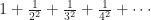 , which converges. (It adds to
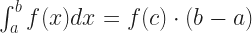
 for values of j from 1 up to N. Or we can bundle all these values together into a vector, and write everything as

 , inside the square where x is between 0 and 2 and y is between 0 and 3. Suppose you had a putative maximum on the inside, like, where x was 1 and y was 2. What happens if you increase x a tiny bit? If you increase y by twice that? No, it’s only on the edges you can get a maximum that can’t be locally bettered. And only on the corners of the edges, at that.
  in it? Could we just say you have a new variable
  that just happens to be equal to the square of y? Will that work? If you have to have the sine of z? Are you sure that z isn’t going to get outside the region where the sine of z is pretty close to just being z? Can you check?
  . This is a general idea. We’re expressing that it maps things in the set D to things in the set R. We can use the notation to write something more specific. If ‘z’ is in the set D, we might write
  . This describes the rule that matches things in the domain to things in the range.
  represents the evaluation of this rule at a specific point, the one where the independent variable has the value ‘2’.
  represents the evaluation of this rule at a specific point without committing to what that point is.
  represents a collection of points. It’s the set you get by evaluating the rule at every point in D.
  doesn’t have any fixed points or shuffled-around points. It sends everything off to infinity.
  has only a fixed point; nothing from it goes off to infinity and nothing’s shuffled back and forth.
  has a fixed point and a lot of points that shuffle back and forth.
  . What is
  . That’s all we need to know about it.
  . Complex-valued functions are worth a lot of study in their own right. Better, they’re easier to study (at the introductory level) than real-valued functions are. This is such a relief to the mathematics major.
  . This all comes in handy.
  is a rational function. It seems too boring to be worth studying, though, and it is. A “rational function” is a function that’s one polynomial divided by another polynomial. This whether they’re real-valued or complex-valued polynomials.
 . The denominator function is
  .
.  . Sometimes
  . I suppose once, in high school, I might have tried
  but I don’t remember what it looked like. If someone’s done, say,
  please write in and let me know what it looks like.
 is raised to the first power, rather than the second or third or such … well, that’s fair. A needle twice as long having twice the chance of crossing a line? That sounds more likely than a needle twice as long having four times the chance, or eight times the chance.
  , there’s still a probability that the needle crosses at least one line. It never becomes certain. No matter how long the needle is it could fall parallel to all the floor lines and miss them all. The probability is instead:
 is the world-famous arcsecant function. That is, it’s whatever angle has as its secant the number


 ? Why not
  ?” is more pleasant, to a certain personality, than pondering what a directrix might be and why we might use one.
  , yes. But it’s more fun.
 then we can find
  . The calculation on the right-hand side of this is easy; double your number and subtract one. Then to the lookup table; find the angle whose cosine is that number. That angle is two times θ. So divide that angle in two. Cosine of that is, well,

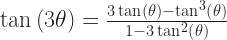
 . Or the cube of the sine of theta, or the cube of the tangent of theta. Whatever. The trouble is I don’t see a way to calculate cosine (sine, tangent) of 3θ, or 3 times the cosine (etc) of θ. Nor to get some other simple expression out of that. I can get mixtures of the cosine of 3θ plus the cosine of θ, sure. But that doesn’t help me figure out what θ is.
 instead. But if you don’t have a log table, and only have a table of cosines, you can calculate
  at least.
  and
and  . Same old boring fixed points. The cosine is a little more interesting. For that we have
  .
.  ). It creeps into problems that don’t look like fixed points. Calculus students learn of something called the Newton-Raphson Iteration. It finds roots, points where a function f(x) equals zero. Mathematics majors learn of numerical methods to solve ordinary differential equations. The most stable of these are again fixed-point iteration schemes, albeit in disguise.


