The handful of comic strips I’ve chosen to write about this week include a couple with characters who want to not be wrong. That’s a common impulse among people learning mathematics, that drive to have the right answer.
Will Henry’s Wallace the Brave for the 8th opens the theme, with Rose excited to go to mathematics camp as a way of learning more ways to be right. I imagine everyone feels this appeal of mathematics, arithmetic particularly. If you follow these knowable rules, and avoid calculation errors, you get results that are correct. Not just coincidentally right, but right for all time. It’s a wonderful sense of security, even when you get past that childhood age where so little is in your control.
A thing that creates a problem, if you love this too closely, is that much of mathematics builds on approximations. Things we know not to be right, but which we know are not too far wrong. You expect this from numerical mathematics, yes. But it happens in analytic mathematics too. I remember struggling in high school physics, in the modeling a pendulum’s swing. To do this you have to approximate the sine of the angle the pendulum bob with the angle itself. This approximation is quite good, if the angle is small, as you can see from comparing the sine of 0.01 radians to the number 0.01. But I wanted to know when that difference was accounted for, and it never was.
(An alternative interpretation is to treat the path swung by the end of the pendulum as though it were part of a parabola, instead of the section of circle that it really is. A small arc of parabola looks much like a small arc of circle. But there is a difference, not accounted for.)
Nor would it be. A regular trick in analytic mathematics is to show that the thing you want is approximated well enough by a thing you can calculate. And then show that if one takes a limit of the thing you can calculate you make the error infinitesimally small. This is all rigorous and you can in time come to accept it. I hope Rose someday handles the discovery that we get to right answers through wrong-but-useful ones well.
Charles Schulz’s Peanuts Begins for the 8th is one that I have featured here before. It’s built on Lucy not accepting that the answer to a multiplication can be zero, even if it is zero times zero. It’s also built on the mixture of meanings between “zero” and “nothing” and “not existent”. Lucy’s right that zero times zero has to be something, as in a thing with some value. But we also so often use zero to mean “nothing that exists” makes zero a struggle to learn and to work with.
Dan Thompson’s Brevity for the 12th is an anthropomorphic numerals joke, built on the ancient playground pun about why six is afraid of seven. And a bit of wordplay about odd and even numbers on top of that. For this I again offer the followup joke that I first heard a couple of years ago. Why was it that 7 ate 9? Because 7 knows to eat 3-squared meals a day!
Lincoln Pierce’s Big Nate for the 14th is a baseball statistics joke. Really a sabermetrics joke. Sabermetrics and other fine-grained sports analysis study at the enormous number of games played, and situations within those games. The goal is to find enough similar situations to make estimates about outcomes. This is through what’s called the “frequentist” interpretation of statistics. That is, if this situation has come up a hundred times before, and it’s led to one particular outcome 85 of those times, then there’s an 85 percent chance of that outcome in this situation.
Baseball is well-posed to set up this sort of analysis. The organized game has always demanded the keeping of box scores, close records of what happened in what order. Other sports can have the same techniques applied, though. It’s not likely that Randy has thrown enough pitches to estimate his chance of giving up a walk-off grand slam. But combine all the little league teams there are, and all the seasons they’ve played? That starts to sound plausible. Doesn’t help the feeling that one was scheduled for a win and then it didn’t happen.
I haven’t had the space yet to finish my Little 2021 A-to-Z, so let me resume playing the hits of past ones. For my first, Summer 2015, one, I picked all the topics myself. This one, Orthogonal, I remember as one of the challenging ones. The challenge was the question put in the first paragraph: why do we have this term, which is so nearly a synonym for “perpendicular”? I didn’t find an answer, then, or since. But I was able to think about how we use “orthogonal” and what it might do that “perpendicular ” doesn’t..
Orthogonal.
Orthogonal is another word for perpendicular. So why do we need another word for that?
It helps to think about why “perpendicular” is a useful way to organize things. For example, we can describe the directions to a place in terms of how far it is north-south and how far it is east-west, and talk about how fast it’s travelling in terms of its speed heading north or south and its speed heading east or west. We can separate the north-south motion from the east-west motion. If we’re lucky these motions separate entirely, and we turn a complicated two- or three-dimensional problem into two or three simpler problems. If they can’t be fully separated, they can often be largely separated. We turn a complicated problem into a set of simpler problems with a nice and easy part plus an annoying yet small hard part.
And this is why we like perpendicular directions. We can often turn a problem into several simpler ones describing each direction separately, or nearly so.
And now the amazing thing. We can separate these motions because the north-south and the east-west directions are at right angles to one another. But we can describe something that works like an angle between things that aren’t necessarily directions. For example, we can describe an angle between things like functions that have the same domain. And once we can describe the angle between two functions, we can describe functions that make right angles between each other.
This means we can describe functions as being perpendicular to one another. An example. On the domain of real numbers from -1 to 1, the function is perpendicular to the function . And when we want to study a more complicated function we can separate the part that’s in the “direction” of f(x) from the part that’s in the “direction” of g(x). We can treat functions, even functions we don’t know, as if they were locations in space. And we can study and even solve for the different parts of the function as if we were pinning down the north-south and the east-west movements of a thing.
So if we want to study, say, how heat flows through a body, we can work out a series of “direction” for functions, and work out the flow in each of those “directions”. These don’t have anything to do with left-right or up-down directions, but the concepts and the convenience is similar.
I’ve spoken about this in terms of functions. But we can define the “angle” between things for many kinds of mathematical structures. Once we can do that, we can have “perpendicular” pairs of things. I’ve spoken only about functions, but that’s because functions are more familiar than many of the mathematical structures that have orthogonality.
Ah, but why call it “orthogonal” rather than “perpendicular”? And I don’t know. The best I can work out is that it feels weird to speak of, say, the cosine function being “perpendicular” to the sine function when you can’t really say either is in any particular direction. “Orthogonal” seems to appeal less directly to physical intuition while still meaning something. But that’s my guess, rather than the verdict of a skilled etymologist.
I owe Iva Sallay thanks for the suggestion of today’s topic. Sallay is a longtime friend of my blog here. And runs the Find the Factors recreational mathematics puzzle site. If you haven’t been following, or haven’t visited before, this is a fun week to step in again. The puzzles this week include (American) Thanksgiving-themed pictures.
Inverse.
When we visit the museum made of a visual artist’s studio we often admire the tools. The surviving pencils and crayons, pens, brushes and such. We don’t often notice the eraser, the correction tape, the unused white-out, or the pages cut into scraps to cover up errors. To do something is to want to undo it. This is as true for the mathematics of a circle as it is for the drawing of one.
If not to undo something, we do often want to know where something comes from. A classic paper asks can one hear the shape of a drum? You hear a sound. Can you say what made that sound? Fine, dismiss the drum shape as idle curiosity. The same question applies to any sensory data. If our hand feels cooler here, where is the insulation of the building damaged? If we have this electrocardiogram reading, what can we say about the action of the heart producing that? If we see the banks of a river, what can we know about how the river floods?
And this is the point, and purpose, of inverses. We can understand them as finding the causes of what we observe.
The first inverse we meet is usually the inverse function. It’s introduced as a way to undo what a function does. That’s an odd introduction, if you’re comfortable with what a function is. A function is a mathematical construct. It’s two sets — a domain and a range — and a rule that links elements in the domain to the range. To “undo” a function is like “undoing” a rectangle. But a function has a compelling “physical” interpretation. It’s routine to introduce functions as machines that take some numbers in and give numbers out. We think of them as ways to transform the domain into the range. In functional analysis get to thinking of domains as the most perfect putty. We expect functions to stretch and rotate and compress and slide along as though they were drawing a Betty Boop cartoon.
So we’re trained to speak of a function as a verb, acting on pieces of the domain. An element or point, or a region, or the whole domain. We think the function “maps”, or “takes”, or “transforms” this into its image in the range. And if we can turn one thing into another, surely we can turn it back.
Some things it’s obvious we can turn back. Suppose our function adds 2 to whatever we give it. We can get the original back by subtracting 2. If the function subtracts 32 and divides by 1.8, we can reverse it by multiplying by 1.8 and adding 32. If the function takes the reciprocal, we can take the reciprocal again. We have a bit of a problem if we started out taking the reciprocal of 0, but who would want to do such a thing anyway? If the function squares a number, we can undo that by taking the square root. Unless we started from a negative number. Then we have trouble.
The trouble is not every function has an inverse. Which we could have realized by thinking how to undo “multiply by zero”. To be a well-defined function, the rule part has to match elements in the domain to exactly one element in the range. This makes the function, in the impenetrable jargon of the mathematician, a “one-to-one function”. Or you can describe it with the more intuitive label of “bijective”.
But there’s no reason more than one thing in the domain can’t match to the same thing in the range. If I know the cosine of my angle is , my angle might be 30 degrees. Or -30 degrees. Or 390 degrees. Or 330 degrees. You may protest there’s no difference between a 30 degree and a 390 degree angle. I agree those angles point in the same direction. But a gear rotated 390 degrees has done something that a gear rotated 30 degrees hasn’t. If all I know is where the dot I’ve put on the gear is, how can I know how much it’s rotated?
So what we do is shift from the actual cosine into one branch of the cosine. By restricting the domain we can create a function that has the same rule as the one we want, but that’s also one-to-one and so has an inverse. What restriction to use? That depends on what you want. But mathematicians have some that come up so often they might as well be defaults. So the square root is the inverse of the square of nonnegative numbers. The inverse Cosine is the inverse of the cosine of angles from 0 to 180 degrees. The inverse Sine is the inverse of the sine of angles from -90 to 90 degrees. The capital letters are convention to say we’re doing this. If we want a different range, we write out that we’re looking for an inverse cosine from -180 to 0 degrees or whatever. (Yes, the mathematician will default to using radians, rather than degrees, for angles. That’s a different essay.) It’s an imperfect solution, but it often works well enough.
The trouble we had with cosines, and functions, continues through all inverses. There are almost always alternate causes. Many shapes of drums sound alike. Take two metal bars. Heat both with a blowtorch, one on the end and one in the center. Not to the point of melting, only to the point of being too hot to touch. Let them cool in insulated boxes for a couple weeks. There’ll be no measurement you can do on the remaining heat that tells you which one was heated on the end and which the center. That’s not because your thermometers are no good or the flow of heat is not deterministic or anything. It’s that both starting cases settle to the same end. So here there is no usable inverse.
This is not to call inverses futile. We can look for what we expect to find useful. We are inclined to find inverses of the cosine between 0 and 180 degrees, even though 4140 through 4320 degrees is as legitimate. We may not know what is wrong with a heart, but have some idea what a heart could do and still beat. And there’s a famous example in 19th-century astronomy. After the discovery of Uranus came the discovery it did not move right. For a while it moved across the sky too fast for its distance from the sun. Then it started moving too slow. The obvious supposition was that there was another, not-yet-seen, planet, affecting its orbit.
The trouble is finding it. Calculating the orbit from what data they had required solving equations with 13 unknown quantities. John Couch Adams and Urbain Le Verrier attempted this anyway, making suppositions about what they could not measure. They made great suppositions. Le Verrier made the better calculations, and persuaded an astronomer (Johann Gottfried Galle, assisted by Heinrich Louis d’Arrest) to go look. Took about an hour of looking. They also made lucky suppositions. Both, for example, supposed the trans-Uranian planet would obey “Bode’s Law”, a seeming pattern in the size of planetary radiuses. The actual Neptune does not. It was near enough in the sky to where the calculated planet would be, though. The world is vaster than our imaginations.
That there are many ways to draw Betty Boop does not mean there’s nothing to learn about how this drawing was done. And so we keep having inverses as a vibrant field of mathematics.
Analysis is about proving why the rest of mathematics works. It’s a hard field. My experience, a typical one, included crashing against real analysis as an undergraduate and again as a graduate student. It turns out mathematics works by throwing a lot of symbols around.
Let me give an example. If you read pop mathematics blogs you know about the number represented by . You’ve seen proofs, some of them even convincing, that this number equals 1. Not a tiny bit less than 1, but exactly 1. Here’s a real-analysis treatment. And — I may regret this — I recommend you don’t read it. Not closely, at least. Instead, look at its shape. Look at the words and symbols as graphic design elements, and trust that what I say is not nonsense. Resume reading after the horizontal rule.
It’s convenient to have a name for the number . I’ll call that , for “repeating”. 1 we’ll call 1. I think you’ll grant that whatever r is, it can’t be more than 1. I hope you’ll accept that if the difference between 1 and r is zero, then r equals 1. So what is the difference between 1 and r?
Give me some number . It has to be a positive number. The implication in the letter is that it’s a small number. This isn’t actually required in general. We expect it. We feel surprise and offense if it’s ever not the case.
I can show that the difference between 1 and r is less than . I know there is some smallest counting number N so that . For example, say is 0.125. Then we can let N = 1, and . Or suppose is 0.00625. But then if N = 3, . (If is bigger than 1, let N = 1.) Now we have to ask why I want this N.
Whatever the value of r is, I know that it is more than 0.9. And that it is more than 0.99. And that it is more than 0.999. In fact, it’s more than the number you get by truncating r after any whole number N of digits. Let me call the number you get by truncating r after N digits. So, and and and so on.
Since , it has to be true that . And since we know what is, we can say exactly what is. It's . And we picked N so that . So . But all we know of is that it's a positive number. It can be any positive number. So has to be smaller than each and every positive number. The biggest number that’s smaller than every positive number is zero. So the difference between 1 and r must be zero and so they must be equal.
That is a compelling argument. Granted, it compels much the way your older brother kneeling on your chest and pressing your head into the ground compels. But this argument gives the flavor of what much of analysis is like.
For one, it is fussy, leaning to technical. You see why the subject has the reputation of driving off all but the most intent mathematics majors. If you get comfortable with this sort of argument it’s hard to notice anymore.
For another, the argument shows that the difference between two things is less than every positive number. Therefore the difference is zero and so the things are equal. This is one of mathematics’ most important tricks. And another point, there’s a lot of talk about . And about finding differences that are, it usually turns out, smaller than some . (As an undergraduate I found something wasteful in how the differences were so often so much less than . We can’t exhaust the small numbers, though. It still feels uneconomic.)
Something this misses is another trick, though. That’s adding zero. I couldn’t think of a good way to use that here. What we often get is the need to show that, say, function and function are equal. That is, that they are less than apart. What we can often do is show that is close to some related function, which let me call .
I know what you’re suspecting: must be a polynomial. Good thought! Although in my experience, it’s actually more likely to be a piecewise constant function. That is, it’s some number, eg, “2”, for part of the domain, and then “2.5” in some other region, with no transition between them. Some other values, even values not starting with “2”, in other parts of the domain. Usually this is easier to prove stuff about than even polynomials are.
But get back to . It’s got the same deal as , some approximation easier to prove stuff about. Then we want to show that is close to some . And then show that is close to . So — watch this trick. Or, again, watch the shape of this trick. Read again after the horizontal rule.
The difference is equal to since adding zero, that is, adding the number , can’t change a quantity. And is equal to . Same reason: is zero. So:
Now we use the “triangle inequality”. If a, b, and c are the lengths of a triangle’s sides, the sum of any two of those numbers is larger than the third. And that tells us:
And then if you can show that is less than ? And that is also ? And you see where this is going for ? Then you’ve shown that . With luck, each of these little pieces is something you can prove.
Don’t worry about what all this means. It’s meant to give a flavor of what you do in an analysis course. It looks hard, but most of that is because it’s a different sort of work than you’d done before. If you hadn’t seen the adding-zero and triangle-inequality tricks? I don’t know how long you’d need to imagine them.
There are other tricks too. An old reliable one is showing that one thing is bounded by the other. That is, that . You use this trick all the time because if you can also show that , then those two have to be equal.
The good thing — and there is good — is that once you get the hang of these tricks analysis starts to come together. And even get easier. The first course you take as a mathematics major is real analysis, all about functions of real numbers. The next course in this track is complex analysis, about functions of complex-valued numbers. And it is easy. Compared to what comes before, yes. But also on its own. Every theorem in complex analysis named after Augustin-Louis Cauchy. They all show that the integral of your function, calculated along a closed loop, is zero. I exaggerate by .
In grad school, if you make it, you get to functional analysis, which examines functions on functions and other abstractions like that. This, too, is easy, possibly because all the basic approaches you’ve seen several courses over. Or it feels easy after all that mucking around with the real numbers.
This is not the entirety of explaining how mathematics works. Since all these proofs depend on how numbers work, we need to show how numbers work. How logic works. But those are subjects we can leave for grad school, for someone who’s survived this gauntlet.
What we mean by that is the area between some left boundary, , and some right boundary, , that’s above the x-axis, and below that curve. And there’s just no finding a, you know, answer. Something that looks like (to make up an answer) the area is or something normal like that. The one interesting exception is that you can find the area if the left bound is and the right bound . That’s done by some clever reasoning and changes of variables which is why we see that and only that in freshman calculus. (Oh, and as a side effect we can get the integral between 0 and infinity, because that has to be half of that.)
Anyway, Quintanilla includes a nice bit along the way, that I don’t remember from my freshman calculus, pointing out why we can’t come up with a nice simple formula like that. It’s a loose argument, showing what would happen if we suppose there is a way to integrate this using normal functions and showing we get a contradiction. A proper proof is much harder and fussier, but this is likely enough to convince someone who understands a bit of calculus and a bit of Taylor series.
Today’s is another topic suggested by Mr Wu, author of the Singapore Maths Tuition blog. The Wronskian is named for Józef Maria Hoëne-Wroński, a Polish mathematician, born in 1778. He served in General Tadeusz Kosciuszko’s army in the 1794 Kosciuszko Uprising. After being captured and forced to serve in the Russian army, he moved to France. He kicked around Western Europe and its mathematical and scientific circles. I’d like to say this was all creative and insightful, but, well. Wikipedia describes him trying to build a perpetual motion machine. Trying to square the circle (also impossible). Building a machine to predict the future. The St Andrews mathematical biography notes his writing a summary of “the general solution of the fifth degree [polynomial] equation”. This doesn’t exist.
Both sources, though, admit that for all that he got wrong, there were flashes of insight and brilliance in his work. The St Andrews biography particularly notes that Wronski’s tables of logarithms were well-designed. This is a hard thing to feel impressed by. But it’s hard to balance information so that it’s compact yet useful. He wrote about the Wronskian in 1812; it wouldn’t be named for him until 1882. This was 29 years after his death, but it does seem likely he’d have enjoyed having a familiar thing named for him. I suspect he wouldn’t enjoy my next paragraph, but would enjoy the fight with me about it.
The Wronskian is a thing put into Introduction to Ordinary Differential Equations courses because students must suffer in atonement for their sins. Those who fail to reform enough must go on to the Hessian, in Partial Differential Equations.
To be more precise, the Wronskian is the determinant of a matrix. The determinant you find by adding and subtracting products of the elements in a matrix together. It’s not hard, but it is tedious, and gets more tedious pretty fast as the matrix gets bigger. (In Big-O notation, it’s the order of the cube of the matrix size. This is rough, for things humans do, although not bad as algorithms go.) The matrix here is made up of a bunch of functions and their derivatives. The functions need to be ones of a single variable. The derivatives, you need first, second, third, and so on, up to one less than the number of functions you have.
If you have two functions, and , you need their first derivatives, and . If you have three functions, , , and , you need first derivatives, , , and , as well as second derivatives, , , and . If you have functions and here I’ll call them , you need derivatives, and so on through . You see right away this is a fun and exciting thing to calculate. Also why in intro to differential equations you only work this out with two or three functions. Maybe four functions if the class has been really naughty.
Go through your functions and your derivatives and make a big square matrix. And then you go through calculating the derivative. This involves a lot of multiplying strings of these derivatives together. It’s a lot of work. But at least doing all this work gets you older.
So one will ask why do all this? Why fit it into every Intro to Ordinary Differential Equations textbook and why slip it in to classes that have enough stuff going on?
One answer is that if the Wronskian is not zero for some values of the independent variable, then the functions that went into it are linearly independent. Mathematicians learn to like sets of linearly independent functions. We can treat functions like directions in space. Linear independence assures us none of these functions are redundant, pointing a way we already can describe. (Real people see nothing wrong in having north, east, and northeast as directions. But mathematicians would like as few directions in our set as possible.) The Wronskian being zero for every value of the independent variable seems like it should tell us the functions are linearly dependent. It doesn’t, not without some more constraints on the functions.
This is fine, but who cares? And, unfortunately, in Intro it’s hard to reach a strong reason to care. To this major, the emphasis on linearly independent functions felt misplaced. It’s the sort of thing we care about in linear algebra. Or some course where we talk about vector spaces. Differential equations do lead us into vector spaces. It’s hard to find a corner of analysis that doesn’t.
Every ordinary differential equation has a secret picture. This is a vector field. One axis in the field is the independent variable of the function. The other axes are the value of the function. And maybe its derivatives, depending on how many derivatives are used in the ordinary differential equation. To solve one particular differential equation is to find one path in this field. People who just use differential equations will want to find one path.
Mathematicians tend to be fine with finding one path. But they want to find what kinds of paths there can be. Are there paths which the differential equation picks out, by making paths near it stay near? Or by making paths that run away from it? And here is the value of the Wronskian. The Wronskian tells us about the divergence of this vector field. This gives us insight to how these paths behave. It’s in the same way that knowing where high- and low-pressure systems are describes how the weather will change. The Wronskian, by way of a thing called Liouville’s Theorem that I haven’t the strength to describe today, ties in to the Hamiltonian. And the Hamiltonian we see in almost every mechanics problem of note.
You can see where the mathematics PhD, or the physicist, would find this interesting. But what about the student, who would look at the symbols evoked by those paragraphs above with reasonable horror?
And here’s the second answer for what the Wronskian is good for. It helps us solve ordinary differential equations. Like, particular ones. An ordinary differential equation will (normally) have several linearly independent solutions. If you know all but one of those solutions, it’s possible to calculate the Wronskian and, from that, the last of the independent solutions. Since a big chunk of mathematics — particularly for science or engineering — is solving differential equations you see why this is something valuable. Allow that it’s tedious. Tedious work we can automate, or give to research assistant to do.
One then asks what kind of differential equation would have all-but-one answer findable, and yield that last one only by long efforts of hard work. So let me show you an example ordinary differential equation:
Here , , and are some functions that depend only on the independent variable, . Don’t know what they are; don’t care. The differential equation is a lot easier of and are constants, but we don’t insist on that.
This equation has a close cousin, and one that’s easier to solve than the original. Is cousin is called a homogeneous equation:
The left-hand-side, the parts with the function that we want to find, is the same. It’s the right-hand-side that’s different, that’s a constant zero. This is what makes the new equation homogenous. This homogenous equation is easier and we can expect to find two functions, and , that solve it. If and are constant this is even easy. Even if they’re not, if you can find one solution, the Wronskian lets you generate the second.
That’s nice for the homogenous equation. But if we care about the original, inhomogenous one? The Wronskian serves us there too. Imagine that the inhomogenous solution has any solution, which we’ll call . (The ‘p’ stands for ‘particular’, as in “the solution for this particular ”.) But also has to solve that inhomogenous differential equation. It seems startling but if you work it out, it’s so. (The key is the derivative of the sum of functions is the same as the sum of the derivative of functions.) also has to solve that inhomogenous differential equation. In fact, for any constants and , it has to be that is a solution.
I’ll skip the derivation; you have Wikipedia for that. The key is that knowing these homogenous solutions, and the Wronskian, and the original , will let you find the that you really want.
My reading is that this is more useful in proving things true about differential equations, rather than particularly solving them. It takes a lot of paper and I don’t blame anyone not wanting to do it. But it’s a wonder that it works, and so well.
Don’t make your instructor so mad you have to do the Wronskian for four functions.
I’m happy to have a subject from Elke Stangl, author of elkemental Force. That’s a fun and wide-ranging blog which, among other things, just published a poem about proofs. You might enjoy.
One delight, and sometimes deadline frustration, of these essays is discovering things I had not thought about. Researching quadratic forms invited the obvious question of what is a form? And that goes undefined on, for example, Mathworld. Also in the textbooks I’ve kept. Even ones you’d think would mention, like R W R Darling’s Differential Forms and Connections, or Frigyes Riesz and Béla Sz-Nagy’s Functional Analysis. Reluctantly I started thinking about what we talk about when discussing forms.
Quadratic forms offer some hints. These take a vector in some n-dimensional space, and return a scalar. Linear forms, and cubic forms, do the same. The pattern suggests a form is a mapping from a space like to or maybe to . That looks good, but then we have to ask: isn’t that just an operator? Also: then what about differential forms? Or volume forms? These are about how to fill space. There’s nothing scalar in that. But maybe these are both called forms because they fill similar roles. They might have as little to do with one another as red pandas and giant pandas do.
Enlightenment comes after much consideration or happening on Wikipedia’s page about homogenous polynomials. That offers “an algebraic form, or simply form, is a function defined by a homogeneous polynomial”. That satisfies. First, because it gets us back to polynomials. Second, because all the forms I could think of do have rules based in homogeneous polynomials. They might be peculiar polynomials. Volume forms, for example, have a polynomial in wedge products of differentials. But it counts.
A function’s homogenous if it scales a particular way. Evaluate it at some set of coordinates x, y, z, (more variables if you need). That’s some number (let’s say). Take all those coordinates and multiply them by the same constant; let me call that α. Evaluate the function at α x, α y α z, (α times more variables if you need). Then that value is αk times the original value of f. k is some constant. It depends on the function, but not on what x, y, z, (more) are.
For a quadratic form, this constant k equals 4. This is because in the quadratic form, all the terms in the polynomial are of the second degree. So, for example, is a quadratic form. So is ; the x times the y brings this to a second degree. Also a quadratic form is . So is .
This can have many variables. If we have a lot, we have a couple choices. One is to start using subscripts, and to write the form something like:
This is respectable enough. People who do a lot of differential geometry get used to a shortcut, the Einstein Summation Convention. In that, we take as implicit the summation instructions. So they’d write the more compact . Those of us who don’t do a lot of differential geometry think that looks funny. And we have more familiar ways to write things down. Like, we can put the collection of variables into an ordered n-tuple. Call it the vector . If we then think to put the numbers into a square matrix we have a great way of writing things. We have to manipulate the a little to make the matrix, but it’s nothing complicated. Once that’s done we can write the quadratic form as:
This uses matrix multiplication. The vector we assume is a column vector, a bunch of rows one column across. Then we have to take its transposition, one row a bunch of columns across, to make the matrix multiplication work out. If we don’t like that notation with its annoying superscripts? We can declare the bare ‘x’ to mean the vector, and use inner products:
This is easier to type at least. But what does it get us?
Looking at some quadratic forms may give us an idea. practically begs to be matched to an , and the name “the equation of a circle”. is less familiar, but to the crowd reading this, not much less familiar. Fill that out to and we have a hyperbola. If we have and let that then we have an ellipse, something a bit wider than it is tall. Similarly is a hyperbola still, just anamorphic.
If we expand into three variables we start to see spheres: just begs to equal . Or ellipsoids: , set equal to some (positive) , is something we might get from rolling out clay. Or hyperboloids: or , set equal to , give us nice shapes. (We can also get cylinders: equalling some positive number describes a tube.)
How about ? This also wants to be an ellipse. , to pick an easy number, is a rotated ellipse. The long axis is along the line described by . The short axis is along the line described by . How about — let me make this easy. ? The equation describes a hyperbola, but a rotated one, with the x- and y-axes as its asymptotes.
Do you want to take any guesses about three-dimensional shapes? Like, what might represent? If you’re thinking “ellipsoid, only it’s at an angle” you’re doing well. It runs really long in one direction, along the plane described by . It runs medium-size along the plane described by . It runs pretty short along the z-axis. We could run some more complicated shapes. Ellipses pointing in weird directions. Hyperboloids of different shapes. They’ll have things in common.
One is that they have obviously important axes. Axes of symmetry, particularly. There’ll be one for each dimension of space. An ellipse has a long axis and a short axis. An ellipsoid has a long, a middle, and a short. (It might be that two of these have the same length. If all three have the same length, you have a sphere, my friend.) A hyperbola, similarly, has two axes of symmetry. One of them is the midpoint between the two branches of the hyperbola. One of them slices through the two branches, through the points where the two legs come closest together. Hyperboloids, in three dimensions, have three axes of symmetry. One of them connects the points where the two branches of hyperboloid come closest together. The other two run perpendicular to that.
We can go on imagining more dimensions of space. We don’t need them. The important things are already there. There are, for these shapes, some preferred directions. The ones around which these quadratic-form shapes have symmetries. These directions are perpendicular to each other. These preferred directions are important. We call them “eigenvectors”, a partly-German name.
Eigenvectors are great for a bunch of purposes. One is that if the matrix A represents a problem you’re interested in? The eigenvectors are probably a great basis to solve problems in it. This is a change of basis vectors, which is the same work as doing a rotation. And it’s happy to report this change of coordinates doesn’t mess up the problem any. We can rewrite the problem to be easier.
And, roughly, any time we look at reflections in a Euclidean space, there’s a quadratic form lurking around. This leads us into interesting places. Looking at reflections encourages us to see abstract algebra, to see groups. That space can be rotated in infinitesimally small pieces gets us a kind of group named a Lie (pronounced ‘lee’) Algebra. Quadratic forms give us a way of classifying those.
Quadratic forms work in number theory also. There’s a neat theorem, the 15 Theorem. If a quadratic form, with integer coefficients, can produce all the integers from 1 through 15, then it can produce all positive numbers. For example, can, for sets of integers x, y, z, and w, add up to any positive number you like. (It’s not guaranteed this will happen. can’t produce 15.) We know of at least 54 combinations which generate all the positive integers, like and and such.
There’s more, of course. There always is. I spent time skimming Quadratic Forms and their Applications, Proceedings of the Conference on Quadratic Forms and their Applications. It was held at University College Dublin in July of 1999. It’s some impressive work. I can think of very little that I can describe. Even Winfried Scharlau’s On the History of the Algebraic Theory of Quadratic Forms, from page 229, is tough going. Ina Kersten’s Biography of Ernst Witt, one of the major influences on quadratic forms, is accessible. I’m not sure how much of the particular work communicates.
It’s easy at least to know what things this field is about, though. The things that we calculate. That they connect to novel and abstract places shows how close together arithmetic and dynamical systems and topology and group theory and number theory are, despite appearances.
Today’s topic suggestion was suggested by bunnydoe. I know of a project bunnydoe runs, but not whether it should be publicized. It is another biographical piece. Biographies and complex numbers, that seems to be the theme of this year.
The exact suggestion I got for L was “Leibniz, the inventor of Calculus”. I can’t in good conscience offer that. This isn’t to deny Leibniz’s critical role in calculus. We rely on many of the ideas he’d had for it. We especially use his notation. But there are few great big ideas that can be truly credited to an inventor, or even a team of inventors. Put aside the sorry and embarrassing priority dispute with Isaac Newton. Many mathematicians in the 16th and 17th century were working on how to improve the Archimedean “method of exhaustion”. This would find the areas inside select curves, integral calculus. Johannes Kepler worked out the areas of ellipse slices, albeit with considerable luck. Gilles Roberval tried working out the area inside a curve as the area of infinitely many narrow rectangular strips. We still learn integration from this. Pierre de Fermat recognized how tangents to a curve could find maximums and minimums of functions. This is a critical piece of differential calculus. Isaac Barrow, Evangelista Torricelli (of barometer fame), Pietro Mengoli, and Stephano Angeli all pushed mathematics towards calculus. James Gregory proved, in geometric form, the relationship between differentiation and integration. That relationship is the Fundamental Theorem of Calculus.
This is not to denigrate Leibniz. We don’t dismiss the Wright Brothers though we know that without them, Alberto Santos-Dumont or Glenn Curtiss or Samuel Langley would have built a workable airplane anyway. We have Leibniz’s note, dated the 29th of October, 1675 (says Florian Cajori), writing out to mean the sum of all l’s. By mid-November he was integrating functions, and writing out his work as . Any mathematics or physics or chemistry or engineering major today would recognize that. A year later he was writing things like , which we’d also understand if not quite care to put that way.
Though we use his notation and his basic tools we don’t exactly use Leibniz’s particular ideas of what calculus means. It’s been over three centuries since he published. It would be remarkable if he had gotten the concepts exactly and in the best of all possible forms. Much of Leibniz’s calculus builds on the idea of a differential. This is a quantity that’s smaller than any positive number but also larger than zero. How does that make sense? George Berkeley argued it made not a lick of sense. Mathematicians frowned, but conceded Berkeley was right. By the mid-19th century they had a rationale for differentials that avoided this weird sort of number.
It’s hard to avoid the differential’s lure. The intuitive appeal of “imagine moving this thing a tiny bit” is always there. In science or engineering applications it’s almost mandatory. Few things we encounter in the real world have the kinds of discontinuity that create logic problems for differentials. Even in pure mathematics, we will look at a differential equation like and rewrite it as . Leibniz’s notation gives us the idea that taking derivatives is some kind of fraction. It isn’t, but in many problems we act as though it were. It works out often enough we forget that it might not.
Better, though. From the 1960s Abraham Robinson and others worked out a different idea of what real numbers are. In that, differentials have a rigorous logical definition. We call the mathematics which uses this “non-standard analysis”. The name tells something of its use. This is not to call it wrong. It’s merely not what we learn first, or necessarily at all. And it is Leibniz’s differentials. 304 years after his death there is still a lot of mathematics he could plausibly recognize.
There is still a lot of still-vital mathematics that he touched directly. Leibniz appears to be the first person to use the term “function”, for example, to describe that thing we’re plotting with a curve. He worked on systems of linear equations, and methods to find solutions if they exist. This technique is now called Gaussian elimination. We see the bundling of the equations’ coefficients he did as building a matrix and finding its determinant. We know that technique, today, as Cramer’s Rule, after Gabriel Cramer. The Japanese mathematician Seki Takakazu had discovered determinants before Leibniz, though.
Leibniz tried to study a thing he called “analysis situs”, which two centuries on would be a name for topology. My reading tells me you can get a good fight going among mathematics historians by asking whether he was a pioneer in topology. So I’ll decline to take a side in that.
In the 1680s he tried to create an algebra of thought, to turn reasoning into something like arithmetic. His goal was good: we see these ideas today as Boolean algebra, and concepts like conjunction and disjunction and negation and the empty set. Anyone studying logic knows these today. He’d also worked in something we can see as symbolic logic. Unfortunately for his reputation, the papers he wrote about that went unpublished until late in the 19th century. By then other mathematicians, like Gottlob Frege and Charles Sanders Peirce, had independently published the same ideas.
We give Leibniz’ name to a particular series that tells us the value of π:
(The Indian mathematician Madhava of Sangamagrama knew the formula this comes from by the 14th century. I don’t know whether Western Europe had gotten the news by the 17th century. I suspect it hadn’t.)
The drawback to using this to figure out digits of π is that it takes forever to use. Taking ten decimal digits of π demands evaluating about five billion terms. That’s not hyperbole; it just takes like forever to get its work done.
Which is something of a theme in Leibniz’s biography. He had a great many projects. Some of them even reached a conclusion. Many did not, and instead sprawled out with great ambition and sometimes insight before getting lost. Consider a practical one: he believed that the use of wind-driven propellers and water pumps could drain flooded mines. (Mines are always flooding.) In principle, he was right. But they all failed. Leibniz blamed deliberate obstruction by administrators and technicians. He even blamed workers afraid that new technologies would replace their jobs. Yet even in this failure he observed and had bracing new thoughts. The geology he learned in the mines project made him hypothesize that the Earth had been molten. I do not know the history of geology well enough to say whether this was significant to that field. It may have been another frustrating moment of insight (lucky or otherwise) ahead of its time but not connected to the mainstream of thought.
Another project, tantalizing yet incomplete: the “stepped reckoner”, a mechanical arithmetic machine. The design was to do addition and subtraction, multiplication and division. It’s a breathtaking idea. It earned him election into the (British) Royal Society in 1673. But it never was quite complete, never getting carries to work fully automatically. He never did finish it, and lost friends with the Royal Society when he moved on to other projects. He had a note describing a machine that could do some algebraic operations. In the 1690s he had some designs for a machine that might, in theory, integrate differential equations. It’s a fantastic idea. At some point he also devised a cipher machine. I do not know if this is one that was ever used in its time.
His greatest and longest-lasting unfinished project was for his employer, the House of Brunswick. Three successive Brunswick rulers were content to let Leibniz work on his many side projects. The one that Ernest Augustus wanted was a history of the Guelf family, in the House of Brunswick. One that went back to the time of Charlemagne or earlier if possible. The goal was to burnish the reputation of the house, which had just become a hereditary Elector of the Holy Roman Empire. (That is, they had just gotten to a new level of fun political intriguing. But they were at the bottom of that level.) Starting from 1687 Leibniz did good diligent work. He travelled throughout central Europe to find archival materials. He studied their context and meaning and relevance. He organized it. What he did not do, by his death in 1716, was write the thing.
It is always difficult to understand another person. Moreso someone you know only through biography. And especially someone who lived in very different times. But I do see a particular an modern personality type here. We all know someone who will work so very hard getting prepared to do a project Right that it never gets done. You might be reading the words of one right now.
Leibniz was a compulsive Society-organizer. He promoted ones in Brandenberg and Berlin and Dresden and Vienna and Saint Petersburg. None succeeded. It’s not obvious why. Leibniz was well-connected enough; he’s known to have over six hundred correspondents. Even for a time of great letter-writing, that’s a lot.
But it does seem like something about him offended others. Failing to complete big projects, like the stepped reckoner or the History of the Guelf family, seems like some of that. Anyone who knows of calculus knows of the dispute about the Newton-versus-Leibniz priority dispute. Grant that Leibniz seems not to have much fueled the quarrel. (And that modern historians agree Leibniz did not steal calculus from Newton.) Just being at the center of Drama causes people to rate you poorly.
There seems like there’s more, though. He was liked, for example, by the Electress Sophia of Hanover and her daughter Sophia Charlotte. These were the mother and the sister of Britain’s King George I. When George I ascended to the British throne he forbade Leibniz coming to London until at least one volume of the history was written. (The restriction seems fair, considering Leibniz was 27 years into the project by then.)
There are pieces in his biography that suggest a person a bit too clever for his own good. His first salaried position, for example, was as secretary to a Nuremberg alchemical society. He did not know alchemy. He passed himself off as deeply learned, though. I don’t blame him. Nobody would ever pass a job interview if they didn’t pretend to have expertise. Here it seems to have worked.
But consider, for example, his peace mission to Paris. Leibniz was born in the last years of the Thirty Years War. In that, the Great Powers of Europe battled each other in the German states. They destroyed Germany with a thoroughness not matched until World War II. Leibniz reasonably feared France’s King Louis XIV had designs on what was left of Germany. So his plan was to sell the French government on a plan of attacking Egypt and, from there, the Dutch East Indies. This falls short of an early-Enlightenment idea of rational world peace and a congress of nations. But anyone who plays grand strategy games recognizes the “let’s you and him fight” scheming. (The plan became irrelevant when France went to war with the Netherlands. The war did rope Brandenberg-Prussia, Cologne, Münster, and the Holy Roman Empire into the mess.)
And I have not discussed Leibniz’s work in philosophy, outside his logic. He’s respected for the theory of monads, part of the long history of trying to explain how things can have qualities. Like many he tried to find a deductive-logic argument about whether God must exist. And he proposed the notion that the world that exists is the most nearly perfect that can possibly be. Everyone has been dragging him for that ever since he said it, and they don’t look ready to stop. It’s an unfair rap, even if it makes for funny spoofs of his writing.
The optimal world may need to be badly defective in some ways. And this recognition inspires a question in me. Obviously Leibniz could come to this realization from thinking carefully about the world. But anyone working on optimization problems knows the more constraints you must satisfy, the less optimal your best-fit can be. Some things you might like may end up being lousy, because the overall maximum is more important. I have not seen anything to suggest Leibniz studied the mathematics of optimization theory. Is it possible he was working in things we now recognize as such, though? That he has notes in the things we would call Lagrange multipliers or such? I don’t know, and would like to know if anyone does.
Leibniz’s funeral was unattended by any dignitary or courtier besides his personal secretary. The Royal Academy and the Berlin Academy of Sciences did not honor their member’s death. His grave was unmarked for a half-century. And yet historians of mathematics, philosophy, physics, engineering, psychology, social science, philology, and more keep finding his work, and finding it more advanced than one would expect. Leibniz’s legacy seems to be one always rising and emerging from shade, but never being quite where it should.
This is a slight thing that crossed my reading yesterday. You might enjoy. The question is a silly one: what’s the “optimal” way to slice banana onto a peanut-butter-and-banana sandwich?
Here’s Ethan Rosenthal’s answer. The specific problem this is put to is silly. The optimal peanut butter and banana sandwich is the one that satisfies your desire for a peanut butter and banana sandwich. However, the approach to the problem demonstrates good mathematics, and numerical mathematics, practices. Particularly it demonstrates defining just what your problem is, and what you mean by “optimal”, and how you can test that. And then developing a numerical model which can optimize it.
And the specific question, how much of the sandwich can you cover with banana slices, one of actual interest. A good number of ideas in analysis involve thinking of cover sets: what is the smallest collection of these things which will completely cover this other thing? Concepts like this give us an idea of how to define area, also, as the smallest number of standard reference shapes which will cover the thing we’re interested in. The basic problem is practical too: if we wish to provide something, and have units like this which can cover some area, how can we arrange them so as to miss as little as possible? Or use as few of the units as possible?
GoldenOj suggested the exponential as a topic. It seemed like a good important topic, but one that was already well-explored by other people. Then I realized I could spend time thinking about something which had bothered me.
In here I write about “the” exponential, which is a bit like writing about “the” multiplication. We can talk about and and many other such exponential functions. One secret of algebra, not appreciated until calculus (or later), is that all these different functions are a single family. Understanding one exponential function lets you understand them all. Mathematicians pick one, the exponential with base e, because we find that convenient. e itself isn’t a convenient number — it’s a bit over 2.718 — but it has some wonderful properties. When I write “the exponential” here, I am looking at this function where we look at .
This piece will have a bit more mathematics, as in equations, than usual. If you like me writing about mathematics more than reading equations, you’re hardly alone. I recommend letting your eyes drop to the next sentence, or at least the next sentence that makes sense. You should be fine.
My professor for real analysis, in grad school, gave us one of those brilliant projects. Starting from the definition of the logarithm, as an integral, prove at least thirty things. They could be as trivial as “the log of 1 is 0”. They could be as subtle as how to calculate the log of one number in a different base. It was a great project for testing what we knew about why calculus works.
And it gives me the structure to write about the exponential function. Anyone reading a pop-mathematics blog about exponentials knows them. They’re these functions that, as the independent variable grows, grow ever-faster. Or that decay asymptotically to zero. Some readers know that, if the independent variable is an imaginary number, the exponential is a complex number too. As the independent variable grows, becoming a bigger imaginary number, the exponential doesn’t grow. It oscillates, a sine wave.
That’s weird. I’d like to see why that makes sense.
To say “why” this makes sense is doomed. It’s like explaining “why” 36 is divisible by three and six and nine but not eight. It follows from what the words we have mean. The “why” I’ll offer is reasons why this strange behavior is plausible. It’ll be a mix of deductive reasoning and heuristics. This is a common blend when trying to understand why a result happens, or why we should accept it.
I’ll start with the definition of the logarithm, as used in real analysis. The natural logarithm, if you’re curious. It has a lot of nice properties. You can use this to prove over thirty things. Here it is:
The “s” is a dummy variable. You’ll never see it in actual use.
So now let me summon into existence a new function. I want to call it g. This is because I’ve worked this out before and I want to label something else as f. There is something coming ahead that’s a bit of a syntactic mess. This is the best way around it that I can find.
Here, ‘c’ is a constant. It might be real. It might be imaginary. It might be complex. I’m using ‘c’ rather than ‘a’ or ‘b’ so that I can later on play with possibilities.
So the alert reader noticed that g(x) here means “take the logarithm of x, and divide it by a constant”. So it does. I’ll need two things built off of g(x), though. The first is its derivative. That’s taken with respect to x, the only variable. Finding the derivative of an integral sounds intimidating but, happy to say, we have a theorem to make this easy. It’s the Fundamental Theorem of Calculus, and it tells us:
We can use the ‘ to denote “first derivative” if a function has only one variable. Saves time to write and is easier to type.
The other thing that I need, and the thing I really want, is the inverse of g. I’m going to call this function f(t). A more common notation would be to write but we already have in the works here. There is a limit to how many little one-stroke superscripts we need above g. This is the tradeoff to using ‘ for first derivatives. But here’s the important thing:
Here, we have some extratextual information. We know the inverse of a logarithm is an exponential. We even have a standard notation for that. We’d write
in any context besides this essay as I’ve set it up.
What I would like to know next is: what is the derivative of f(t)? This sounds impossible to know, if we’re thinking of “the inverse of this integration”. It’s not. We have the Inverse Function Theorem to come to our aid. We encounter the Inverse Function Theorem briefly, in freshman calculus. There we use it to do as many as two problems and then hide away forever from the Inverse Function Theorem. (This is why it’s not mentioned in my quick little guide to how to take derivatives.) It reappears in real analysis for this sort of contingency. The inverse function theorem tells us, if f the inverse of g, that:
That g'(f(t)) means, use the rule for g'(x), with f(t) substituted in place of ‘x’. And now we see something magic:
And that is the wonderful thing about the exponential. Its derivative is a constant times its original value. That alone would make the exponential one of mathematics’ favorite functions. It allows us, for example, to transform differential equations into polynomials. (If you want everlasting fame, albeit among mathematicians, invent a new way to turn differential equations into polynomials.) Because we could turn, say,
into
and then
by supposing that f(t) has to be for the correct value of c. Then all you need do is find a value of ‘c’ that makes that last equation true.
Supposing that the answer has this convenient form may remind you of searching for the lost keys over here where the light is better. But we find so many keys in this good light. If you carry on in mathematics you will never stop seeing this trick, although it may be disguised.
In part because it’s so easy to work with. In part because exponentials like this cover so much of what we might like to do. Let’s go back to looking at the derivative of the exponential function.
There are many ways to understand what a derivative is. One compelling way is to think of it as the rate of change. If you make a tiny change in t, how big is the change in f(t)? So what is the rate of change here?
We can pose this as a pretend-physics problem. This lets us use our physical intuition to understand things. This also is the transition between careful reasoning and ad-hoc arguments. Imagine a particle that, at time ‘t’, is at the position . What is its velocity? That’s the first derivative of its position, so, .
If we are using our physics intuition to understand this it helps to go all the way. Where is the particle? Can we plot that? … Sure. We’re used to matching real numbers with points on a number line. Go ahead and do that. Not to give away spoilers, but we will want to think about complex numbers too. Mathematicians are used to matching complex numbers with points on the Cartesian plane, though. The real part of the complex number matches the horizontal coordinate. The imaginary part matches the vertical coordinate.
So how is this particle moving?
To say for sure we need some value of t. All right. Pick your favorite number. That’s our t. f(t) follows from whatever your t was. What’s interesting is that the change also depends on c. There’s a couple possibilities. Let me go through them.
First, what if c is zero? Well, then the definition of g(t) was gibberish and we can’t have that. All right.
What if c is a positive real number? Well, then, f'(t) is some positive multiple of whatever f(t) was. The change is “away from zero”. The particle will push away from the origin. As t increases, f(t) increases, so it pushes away faster and faster. This is exponential growth.
What if c is a negative real number? Well, then, f'(t) is some negative multiple of whatever f(t) was. The change is “towards zero”. The particle pulls toward the origin. But the closer it gets the more slowly it approaches. If t is large enough, f(t) will be so tiny that is too small to notice. The motion declines into imperceptibility.
What if c is an imaginary number, though?
So let’s suppose that c is equal to some real number b times , where .
I need some way to describe what value f(t) has, for whatever your pick of t was. Let me say it’s equal to , where and are some real numbers whose value I don’t care about. What’s important here is that .
And, then, what’s the first derivative? The magnitude and direction of motion? That’s easy to calculate; it’ll be . This is an interesting complex number. Do you see what’s interesting about it? I’ll get there next paragraph.
So f(t) matches some point on the Cartesian plane. But f'(t), the direction our particle moves with a small change in t, is another poiat whatever complex number f'(t) is as another point on the plane. The line segment connecting the origin to f(t) is perpendicular to the one connecting the origin to f'(t). The ‘motion’ of this particle is perpendicular to its position. And it always is. There’s several ways to show this. An easy one is to just pick some values for and and b and try it out. This proof is not rigorous, but it is quick and convincing.
If your direction of motion is always perpendicular to your position, then what you’re doing is moving in a circle around the origin. This we pick up in physics, but it applies to the pretend-particle moving here. The exponentials of and and will all be points on a locus that’s a circle centered on the origin. The values will look like the cosine of an angle plus times the sine of an angle.
And there, I think, we finally get some justification for the exponential of an imaginary number being a complex number. And for why exponentials might have anything to do with cosines and sines.
You might ask what if c is a complex number, if it’s equal to for some real numbers a and b. In this case, you get spirals as t changes. If a is positive, you get points spiralling outward as t increases. If a is negative, you get points spiralling inward toward zero as t increases. If b is positive the spirals go counterclockwise. If b is negative the spirals go clockwise. is the same as .
This does depend on knowing the exponential of a sum of terms, such as of , is equal to the product of the exponential of those terms. This is a good thing to have in your portfolio. If I remember right, it comes in around the 25th thing. It’s an easy result to have if you already showed something about the logarithms of products.
Today’s A To Z term is one I’ve mentioned previously, including in this A to Z sequence. But it was specifically nominated by Goldenoj, whom I know I follow on Twitter. I’m sorry not to be able to give you an account; I haven’t been able to use my @nebusj account for several months now. Well, if I do get a Twitter, Mathstodon, or blog account I’ll refer you there.
An operator is a function. An operator has a domain that’s a space. Its range is also a space. It can be the same space but doesn’t have to be. It is very common for these spaces to be “function spaces”. So common that if you want to talk about an operator that isn’t dealing with function spaces it’s good form to warn your audience. Everything in a particular function space is a real-valued and continuous function. Also everything shares the same domain as everything else in that particular function space.
So here’s what I first wonder: why call this an operator instead of a function? I have hypotheses and an unwillingness to read the literature. One is that maybe mathematicians started saying “operator” a long time ago. Taking the derivative, for example, is an operator. So is taking an indefinite integral. Mathematicians have been doing those for a very long time. Longer than we’ve had the modern idea of a function, which is this rule connecting a domain and a range. So the term might be a fossil.
My other hypothesis is the one I’d bet on, though. This hypothesis is that there is a limit to how many different things we can call “the function” in one sentence before the reader rebels. I felt bad enough with that first paragraph. Imagine parsing something like “the function which the Laplacian function took the function to”. We are less likely to make dumb mistakes if we have different names for things which serve different roles. This is probably why there is another word for a function with domain of a function space and range of real or complex-valued numbers. That is a “functional”. It covers things like the norm for measuring a function’s size. It also covers things like finding the total energy in a physics problem.
I’ve mentioned two operators that anyone who’d read a pop mathematics blog has heard of, the differential and the integral. There are more. There are so many more.
Many of them we can build from the differential and the integral. Many operators that we care to deal with are linear, which is how mathematicians say “good”. But both the differential and the integral operators are linear, which lurks behind many of our favorite rules. Like, allow me to call from the vasty deep functions ‘f’ and ‘g’, and scalars ‘a’ and ‘b’. You know how the derivative of the function is a times the derivative of f plus b times the derivative of g? That’s the differential operator being all linear on us. Similarly, how the integral of is a times the integral of f plus b times the integral of g? Something mathematical with the adjective “linear” is giving us at least some solid footing.
I’ve mentioned before that a wonder of functions is that most things you can do with numbers, you can also do with functions. One of those things is the premise that if numbers can be the domain and range of functions, then functions can be the domain and range of functions. We can do more, though.
One of the conceptual leaps in high school algebra is that we start analyzing the things we do with numbers. Like, we don’t just take the number three, square it, multiply that by two and add to that the number three times four and add to that the number 1. We think about what if we take any number, call it x, and think of . And what if we make equations based on doing this ; what values of x make those equations true? Or tell us something interesting?
Operators represent a similar leap. We can think of functions as things we manipulate, and think of those manipulations as a particular thing to do. For example, let me come up with a differential expression. For some function u(x) work out the value of this:
Let me join in the convention of using ‘D’ for the differential operator. Then we can rewrite this expression like so:
Suddenly the differential equation looks a lot like a polynomial. Of course it does. Remember that everything in mathematics is polynomials. We get new tools to solve differential equations by rewriting them as operators. That’s nice. It also scratches that itch that I think everyone in Intro to Calculus gets, of wanting to somehow see as if it were a square of . It’s not, and is not the square of . It’s composing with itself. But it looks close enough to squaring to feel comfortable.
Nobody needs to do except to learn some stuff about operators. But you might imagine a world where we did this process all the time. If we did, then we’d develop shorthand for it. Maybe a new operator, call it T, and define it that . You see the grammar of treating functions as if they were real numbers becoming familiar. You maybe even noticed the ‘1’ sitting there, serving as the “identity operator”. You know how you’d write out if you needed to write it in full.
But there are operators that we use all the time. These do get special names, and often shorthand. For example, there’s the gradient operator. This applies to any function with several independent variables. The gradient has a great physical interpretation if the variables represent coordinates of space. If they do, the gradient of a function at a point gives us a vector that describes the direction in which the function increases fastest. And the size of that gradient — a functional on this operator — describes how fast that increase is.
The gradient itself defines more operators. These have names you get very familiar with in Vector Calculus, with names like divergence and curl. These have compelling physical interpretations if we think of the function we operate on as describing a moving fluid. A positive divergence means fluid is coming into the system; a negative divergence, that it is leaving. The curl, in fluids, describe how nearby streams of fluid move at different rate.
Physical interpretations are common in operators. This probably reflects how much influence physics has on mathematics and vice-versa. Anyone studying quantum mechanics gets familiar with a host of operators. These have comfortable names like “position operator” or “momentum operator” or “spin operator”. These are operators that apply to the wave function for a problem. They transform the wave function into a probability distribution. That distribution describes what positions or momentums or spins are likely, how likely they are. Or how unlikely they are.
They’re not all physical, though. Or not purely physical. Many operators are useful because they are powerful mathematical tools. There is a variation of the Fourier series called the Fourier transform. We can interpret this as an operator. Suppose the original function started out with time or space as its independent variable. This often happens. The Fourier transform operator gives us a new function, one with frequencies as independent variable. This can make the function easier to work with. The Fourier transform is an integral operator, by the way, so don’t go thinking everything is a complicated set of derivatives.
Another integral-based operator that’s important is the Laplace transform. This is a great operator because it turns differential equations into algebraic equations. Often, into polynomials. You saw that one coming.
This is all a lot of good press for operators. Well, they’re powerful tools. They help us to see that we can manipulate functions in the ways that functions let us manipulate numbers. It should sound good to realize there is much new that you can do, and you already know most of what’s needed to do it.
Today’s A To Z term is another free choice. So I’m picking a term from the world of … mathematics. There are a lot of norms out there. Many are specialized to particular roles, such as looking at complex-valued numbers, or vectors, or matrices, or polynomials.
Still they share things in common, and that’s what this essay is for. And I’ve brushed up against the topic before.
The norm, also, has nothing particular to do with “normal”. “Normal” is an adjective which attaches to every noun in mathematics. This is security for me as while these A-To-Z sequences may run out of X and Y and W letters, I will never be short of N’s.
A “norm” is the size of whatever kind of thing you’re working with. You can see where this is something we look for. It’s easy to look at two things and wonder which is the smaller.
There are many norms, even for one set of things. Some seem compelling. For the real numbers, we usually let the absolute value do this work. By “usually” I mean “I don’t remember ever seeing a different one except from someone introducing the idea of other norms”. For a complex-valued number, it’s usually the square root of the sum of the square of the real part and the square of the imaginary coefficient. For a vector, it’s usually the square root of the vector dot-product with itself. (Dot product is this binary operation that is like multiplication, if you squint, for vectors.) Again, these, the “usually” means “always except when someone’s trying to make a point”.
Which is why we have the convention that there is a “the norm” for a kind of operation. The norm dignified as “the” is usually the one that looks as much as possible like the way we find distances between two points on a plane. I assume this is because we bring our intuition about everyday geometry to mathematical structures. You know how it is. Given an infinity of possible choices we take the one that seems least difficult.
Every sort of thing which can have a norm, that I can think of, is a vector space. This might be my failing imagination. It may also be that it’s quite easy to have a vector space. A vector space is a collection of things with some rules. Those rules are about adding the things inside the vector space, and multiplying the things in the vector space by scalars. These rules are not difficult requirements to meet. So a lot of mathematical structures are vector spaces, and the things inside them are vectors.
A norm is a function that has these vectors as its domain, and the non-negative real numbers as its range. And there are three rules that it has to meet. So. Give me a vector ‘u’ and a vector ‘v’. I’ll also need a scalar, ‘a. Then the function f is a norm when:
. This is a famous rule, called the triangle inequality. You know how in a triangle, the sum of the lengths of any two legs is greater than the length of the third leg? That’s the rule at work here.
. This doesn’t have so snappy a name. Sorry. It’s something about being homogeneous, at least.
If then u has to be the additive identity, the vector that works like zero does.
Norms take on many shapes. They depend on the kind of thing we measure, and what we find interesting about those things. Some are familiar. Look at a Euclidean space, with Cartesian coordinates, so that we might write something like (3, 4) to describe a point. The “the norm” for this, called the Euclidean norm or the L2 norm, is the square root of the sum of the squares of the coordinates. So, 5. But there are other norms. The L1 norm is the sum of the absolute values of all the coefficients; here, 7. The L∞ norm is the largest single absolute value of any coefficient; here, 4.
A polynomial, meanwhile? Write it out as . Take the absolute value of each of these terms. Then … you have choices. You could take those absolute values and add them up. That’s the L1 polynomial norm. Take those absolute values and square them, then add those squares, and take the square root of that sum. That’s the L2 norm. Take the largest absolute value of any of these coefficients. That’s the L∞ norm.
These don’t look so different, even though points in space and polynomials seem to be different things. We designed the tool. We want it not to be weirder than it has to be. When we try to put a norm on a new kind of thing, we look for a norm that resembles the old kind of thing. For example, when we want to define the norm of a matrix, we’ll typically rely on a norm we’ve already found for a vector. At least to set up the matrix norm; in practice, we might do a calculation that doesn’t explicitly use a vector’s norm, but gives us the same answer.
If we have a norm for some vector space, then we have an idea of distance. We can say how far apart two vectors are. It’s the norm of the difference between the vectors. This is called defining a metric on the vector space. A metric is that sense of how far apart two things are. What keeps a norm and a metric from being the same thing is that it’s possible to come up with a metric that doesn’t match any sensible norm.
It’s always possible to use a norm to define a metric, though. Doing that promotes our normed vector space to the dignified status of a “metric space”. Many of the spaces we find interesting enough to work in are such metric spaces. It’s hard to think of doing without some idea of size.
Today’s A To Z term is a free pick. I didn’t notice any suggestions for a mathematics term starting with this letter. I apologize if you did submit one and I missed it. I don’t mean any insult.
What I’ve picked is a concept from analysis. I’ve described this casually as the study of why calculus works. That’s a good part of what it is. Analysis is also about why real numbers work. Later on you also get to why complex numbers and why functions work. But it’s in the courses about Real Analysis where a mathematics major can expect to find the infimum, and it’ll stick around on the analysis courses after that.
The infimum is the thing you mean when you say “lower bound”. It applies to a set of things that you can put in order. The order has to work the way less-than-or-equal-to works with whole numbers. You don’t have to have numbers to put a number-like order on things. Otherwise whoever made up the Alphabet Song was fibbing to us all. But starting out with numbers can let you get confident with the idea, and we’ll trust you can go from numbers to other stuff, in case you ever need to.
A lower bound would start out meaning what you’d imagine if you spoke English. Let me call it L. It’ll make my sentences so much easier to write. Suppose that L is less than or equal to all the elements in your set. Then, great! L is a lower bound of your set.
You see the loophole here. It’s in the article “a”. If L is a lower bound, then what about L – 1? L – 10? L – 1,000,000,000½? Yeah, they’re all lower bounds, too. There’s no end of lower bounds. And that is not what you mean be a lower bound, in everyday language. You mean “the smallest thing you have to deal with”.
But you can’t just say “well, the lower bound of a set is the smallest thing in the set”. There’s sets that don’t have a smallest thing. The iconic example is positive numbers. No positive number can be a lower bound of this. All the negative numbers are lowest bounds of this. Zero can be a lower bound of this.
For the postive numbers, it’s obvious: zero is the lower bound we want. It’s smaller than all of the positive numbers. And there’s no greater number that’s also smaller than all the positive numbers. So this is the infimum of the positive numbers. It’s the greatest lower bound of the set.
The infimum of a set may or may not be part of the original set. But. Between the infimum of a set and the infimum plus any positive number, however tiny that is? There’s always at least one thing in the set.
And there isn’t always an infimum. This is obvious if your set is, like, the set of all the integers. If there’s no lower bound at all, there can’t be a greatest lower bound. So that’s obvious enough.
Infimums turn up in a good number of proofs. There are a couple reasons they do. One is that we want to prove a boundary between two kinds of things exist. It’s lurking in the proof, for example, of the intermediate value theorem. This is the proposition that if you have a continuous function on the domain [a, b], and range of real numbers, and pick some number g that’s between f(a) and f(b)? There’ll be at least one point c, between a and b, where f(c) equals g. You can structure this: look at the set of numbers x in the domain [a, b] whose f(x) is larger than g. So what’s the infimum of this set? What does f have to be for that infimum?
It also turns up a lot in proofs about calculus. Proofs about functions, particularly, especially integrating functions. A proof like this will, generically, not deal with the original function, which might have all kinds of unpleasant aspects. Instead it’ll look at a sequence of approximations of the original function. Each approximation is chosen so it has no unpleasant aspect. And then prove that we could make arbitrarily tiny the difference between the result for the function we want and the result for the sequence of functions we make. Infimums turn up in this, since we’ll want a minimum function without being sure that the minimum is in the sequence we work with.
This is the terminology of stuff to work as lower bounds. There’s a similar terminology to work with upper bounds. The upper-bound equivalent of the infimum is the supremum. They’re abbreviated as inf and sup. The supremum turns up most every time an infimum does, and for the reasons you’d expect.
If an infimum does exist, it’s unique; there can’t be two different ones. Same with the supremum.
And things can get weird. It’s possible to have lower bounds but no infimum. This seems bizarre. This is because we’ve been relying on the real numbers to guide our intuition. And the real numbers have a useful property called being “complete”. So let me break the real numbers. Imagine the real numbers except for zero. Call that the set R’. Now look at the set of positive numbers inside R’. What’s the infimum of the positive numbers, within R’? All we can do is shrug and say there is none, even though there are plenty of lower bounds. The infimum of a set depends on the set. It also depends on what bigger set that the set is within. That something depends both on a set and what the bigger set of things is, is another thing that turns up all the time in analysis. It’s worth becoming familiar with.
Fourier series are named for Jean-Baptiste Joseph Fourier, and are maybe the greatest example of the theory that’s brilliantly wrong. Anyone can be wrong about something. There’s genius in being wrong in a way that gives us good new insights into things. Fourier series were developed to understand how the fluid we call “heat” flows through and between objects. Heat is not a fluid. So what? Pretending it’s a fluid gives us good, accurate results. More, you don’t need to use Fourier series to work with a fluid. Or a thing you’re pretending is a fluid. It works for lots of stuff. The Fourier series method challenged assumptions mathematicians had made about how functions worked, how continuity worked, how differential equations worked. These problems could be sorted out. It took a lot of work. It challenged and expended our ideas of functions.
Fourier also managed to hold political offices in France during the Revolution, the Consulate, the Empire, the Bourbon Restoration, the Hundred Days, and the Second Bourbon Restoration without getting killed for his efforts. If nothing else this shows the depth of his talents.
So, how do you solve differential equations? As long as they’re linear? There’s usually something we can do. This is one approach. It works well. It has a bit of a weird setup.
The weirdness of the setup: you want to think of functions as points in space. The allegory is rather close. Think of the common association between a point in space and the coordinates that describe that point. Pretend those are the same thing. Then you can do stuff like add points together. That is, take the coordinates of both points. Add the corresponding coordinates together. Match that sum-of-coordinates to a point. This gives us the “sum” of two points. You can subtract points from one another, again by going through their coordinates. Multiply a point by a constant and get a new point. Find the angle between two points. (This is the angle formed by the line segments connecting the origin and both points.)
Functions can work like this. You can add functions together and get a new function. Subtract one function from another. Multiply a function by a constant. It’s even possible to describe an “angle” between two functions. Mathematicians usually call that the dot product or the inner product. But we will sometimes call two functions “orthogonal”. That means the ordinary everyday meaning of “orthogonal”, if anyone said “orthogonal” in ordinary everyday life.
We can take equations of a bunch of variables and solve them. Call the values of that solution the coordinates of a point. Then we talk about finding the point where something interesting happens. Or the points where something interesting happens. We can do the same with differential equations. This is finding a point in the space of functions that makes the equation true. Maybe a set of points. So we can find a function or a family of functions solving the differential equation.
You have reasons for skepticism, even if you’ll grant me treating functions as being like points in space. You might remember solving systems of equations. You need as many equations as there are dimensions of space; a two-dimensional space needs two equations. A three-dimensional space needs three equations. You might have worked four equations in four variables. You were threatened with five equations in five variables if you didn’t all settle down. You’re not sure how many dimensions of space “all the possible functions” are. It’s got to be more than the one differential equation we started with.
This is fair. The approach I’m talking about uses the original differential equation, yes. But it breaks it up into a bunch of linear equations. Enough linear equations to match the space of functions. We turn a differential equation into a set of linear equations, a matrix problem, like we know how to solve. So that settles that.
So suppose solves the differential equation. Here I’m going to pretend that the function has one independent variable. Many functions have more than this. Doesn’t matter. Everything I say here extends into two or three or more independent variables. It takes longer and uses more symbols and we don’t need that. The thing about is that we don’t know what it is, but would quite like to.
What we’re going to do is choose a reference set of functions that we do know. Let me call them going on to however many we need. It can be infinitely many. It certainly is at least up to some for some big enough whole number N. These are a set of “basis functions”. For any function we want to represent we can find a bunch of constants, called coefficients. Let me use to represent them. Any function we want is the sum of the coefficient times the matching basis function. That is, there’s some coefficients so that
is true. That summation goes on until we run out of basis functions. Or it runs on forever. This is a great way to solve linear differential equations. This is because we know the basis functions. We know everything we care to know about them. We know their derivatives. We know everything on the right-hand side except the coefficients. The coefficients matching any particular function are constants. So the derivatives of , written as the sum of coefficients times basis functions, are easy to work with. If we need second or third or more derivatives? That’s no harder to work with.
You may know something about matrix equations. That is that solving them takes freaking forever. The bigger the equation, the more forever. If you have to solve eight equations in eight unknowns? If you start now, you might finish in your lifetime. For this function space? We need dozens, hundreds, maybe thousands of equations and as many unknowns. Maybe infinitely many. So we seem to have a solution that’s great apart from how we can’t use it.
Except. What if the equations we have to solve are all easy? If we have to solve a bunch that looks like, oh, and and … well, that’ll take some time, yes. But not forever. Great idea. Is there any way to guarantee that?
It’s in the basis functions. If we pick functions that are orthogonal, or are almost orthogonal, to each other? Then we can turn the differential equation into an easy matrix problem. Not as easy as in the last paragraph. But still, not hard.
So what’s a good set of basis functions?
And here, about 800 words later than everyone was expecting, let me introduce the sine and cosine functions. Sines and cosines make great basis functions. They don’t grow without bounds. They don’t dwindle to nothing. They’re easy to differentiate. They’re easy to integrate, which is really special. Most functions are hard to integrate. We even know what they look like. They’re waves. Some have long wavelengths, some short wavelengths. But waves. And … well, it’s easy to make sets of them orthogonal.
We have to set some rules. The first is that each of these sine and cosine basis functions have a period. That is, after some time (or distance), they repeat. They might repeat before that. Most of them do, in fact. But we’re guaranteed a repeat after no longer than some period. Call that period ‘L’.
Each of these sine and cosine basis functions has to have a whole number of complete oscillations within the period L. So we can say something about the sine and cosine functions. They have to look like these:
Here ‘j’ and ‘k’ are some whole numbers. I have two sets of basis functions at work here. Don’t let that throw you. We could have labelled them all as , with some clever scheme that told us for a given k whether it represents a sine or a cosine. It’s less hard work if we have s’s and c’s. And if we have coefficients of both a’s and b’s. That is, we suppose the function is:
This, at last, is the Fourier series. Each function has its own series. A “series” is a summation. It can be of finitely many terms. It can be of infinitely many. Often infinitely many terms give more interesting stuff. Like this, for example. Oh, and there’s a bare there, not multiplied by anything more complicated. It makes life easier. It lets us see that the Fourier series for, like, 3 + f(x) is the same as the Fourier series for f(x), except for the leading term. The ½ before that makes easier some work that’s outside the scope of this essay. Accept it as one of the merry, wondrous appearances of ‘2’ in mathematics expressions.
It’s great for solving differential equations. It’s also great for encryption. The sines and the cosines are standard functions, after all. We can send all the information we need to reconstruct a function by sending the coefficients for it. This can also help us pick out signal from noise. Noise has a Fourier series that looks a particular way. If you take the coefficients for a noisy signal and remove that? You can get a good approximation of the original, noiseless, signal.
This all seems great. That’s a good time to feel skeptical. First, like, not everything we want to work with looks like waves. Suppose we need a function that looks like a parabola. It’s silly to think we can add a bunch of sines and cosines and get a parabola. Like, a parabola isn’t periodic, to start with.
So it’s not. To use Fourier series methods on something that’s not periodic, we use a clever technique: we tell a fib. We declare that the period is something bigger than we care about. Say the period is, oh, ten million years long. A hundred light-years wide. Whatever. We trust that the difference between the function we do want, and the function that we calculate, will be small. We trust that if someone ten million years from now and a hundred light-years away wishes to complain about our work, we will be out of the office that day. Letting the period L be big enough is a good reliable tool.
The other thing? Can we approximate any function as a Fourier series? Like, at least chunks of parabolas? Polynomials? Chunks of exponential growths or decays? What about sawtooth functions, that rise and fall? What about step functions, that are constant for a while and then jump up or down?
The answer to all these questions is “yes,” although drawing out the word and raising a finger to say there are some issues we have to deal with. One issue is that most of the time, we need an infinitely long series to represent a function perfectly. This is fine if we’re trying to prove things about functions in general rather than solve some specific problem. It’s no harder to write the sum of infinitely many terms than the sum of finitely many terms. You write an ∞ symbol instead of an N in some important places. But if we want to solve specific problems? We probably want to deal with finitely many terms. (I hedge that statement on purpose. Sometimes it turns out we can find a formula for all the infinitely many coefficients.) This will usually give us an approximation of the we want. The approximation can be as good as we want, but to get a better approximation we need more terms. Fair enough. This kind of tradeoff doesn’t seem too weird.
Another issue is in discontinuities. If jumps around? If it has some point where it’s undefined? If it has corners? Then the Fourier series has problems. Summing up sines and cosines can’t give us a sudden jump or a gap or anything. Near a discontinuity, the Fourier series will get this high-frequency wobble. A bigger jump, a bigger wobble. You may not blame the series for not representing a discontinuity. But it does mean that what is, otherwise, a pretty good match for the you want gets this region where it stops being so good a match.
That’s all right. These issues aren’t bad enough, or unpredictable enough, to keep Fourier series from being powerful tools. Even when we find problems for which sines and cosines are poor fits, we use this same approach. Describe a function we would like to know as the sums of functions we choose to work with. Fourier series are one of those ideas that helps us solve problems, and guides us to new ways to solve problems.
The thing most important to know about differential equations is that for short, we call it “diff eq”. This is pronounced “diffy q”. It’s a fun name. People who aren’t taking mathematics smile when they hear someone has to get to “diffy q”.
Sometimes we need to be more exact. Then the less exciting names “ODE” and “PDE” get used. The meaning of the “DE” part is an easy guess. The meaning of “O” or “P” will be clear by the time this essay’s finished. We can find approximate answers to differential equations by computer. This is known generally as “numerical solutions”. So you will encounter talk about, say, “NSPDE”. There’s an implied “of” between the S and the P there. I don’t often see “NSODE”. For some reason, probably a quite arbitrary historical choice, this is just called “numerical integration” instead.
One of algebra’s unsettling things is the idea that we can work with numbers without knowing their values. We can give them names, like ‘x’ or ‘a’ or ‘t’. We can know things about them. Often it’s equations telling us these things. We can make collections of numbers based on them all sharing some property. Often these things are solutions to equations. We can even describe changing those collections according to some rule, even before we know whether any of the numbers is 2. Often these things are functions, here matching one set of numbers to another.
One of analysis’s unsettling things is the idea that most things we can do with numbers we can also do with functions. We can give them names, like ‘f’ and ‘g’ and … ‘F’. That’s easy enough. We can add and subtract them. Multiply and divide. This is unsurprising. We can measure their sizes. This is odd but, all right. We can know things about functions even without knowing exactly what they are. We can group together collections of functions based on some properties they share. This is getting wild. We can even describe changing these collections according to some rule. This change is itself a function, but it is usually called an “operator”, saving us some confusion.
So we can describe a function in an equation. We may not know what f is, but suppose we know is true. We can suppose that if we cared we could find what function, or functions, f made that equation true. There is shorthand here. A function has a domain, a range, and a rule. The equation part helps us find the rule. The domain and range we get from the problem. Or we take the implicit rule that both are the biggest sets of real-valued numbers for which the rule parses. Sometimes biggest sets of complex-valued numbers. We get so used to saying “the function” to mean “the rule for the function” that we’ll forget to say that’s what we’re doing.
There are things we can do with functions that we can’t do with numbers. Or at least that are too boring to do with numbers. The most important here is taking derivatives. The derivative of a function is another function. One good way to think of a derivative is that it describes how a function changes when its variables change. (The derivative of a number is zero, which is boring except when it’s also useful.) Derivatives are great. You learn them in Intro Calculus, and there are a bunch of rules to follow. But follow them and you can pretty much take the derivative of any function even if it’s complicated. Yes, you might have to look up what the derivative of the arc-hyperbolic-secant is. Nobody has ever used the arc-hyperbolic-secant, except to tease a student.
And the derivative of a function is itself a function. So you can take a derivative again. Mathematicians call this the “second derivative”, because we didn’t expect someone would ask what to call it and we had to say something. We can take the derivative of the second derivative. This is the “third derivative” because by then changing the scheme would be awkward. If you need to talk about taking the derivative some large but unspecified number of times, this is the n-th derivative. Or m-th, if you’ve already used ‘n’ to mean something else.
And now we get to differential equations. These are equations in which we describe a function using at least one of its derivatives. The original function, that is, f, usually appears in the equation. It doesn’t have to, though.
We divide the earth naturally (we think) into two pairs of hemispheres, northern and southern, eastern and western. We divide differential equations naturally (we think) into two pairs of two kinds of differential equations.
The first division is into linear and nonlinear equations. I’ll describe the two kinds of problem loosely. Linear equations are the kind you don’t need a mathematician to solve. If the equation has solutions, we can write out procedures that find them, like, all the time. A well-programmed computer can solve them exactly. Nonlinear equations, meanwhile, are the kind no mathematician can solve. They’re just too hard. There’s no processes that are sure to find an answer.
You may ask. We don’t need mathematicians to solve linear equations. Mathematicians can’t solve nonlinear ones. So what do we need mathematicians for? The answer is that I exaggerate. Linear equations aren’t quite that simple. Nonlinear equations aren’t quite that hopeless. There are nonlinear equations we can solve exactly, for example. This usually involves some ingenious transformation. We find a linear equation whose solution guides us to the function we do want.
And that is what mathematicians do in such a field. A nonlinear differential equation may, generally, be hopeless. But we can often find a linear differential equation which gives us insight to what we want. Finding that equation, and showing that its answers are relevant, is the work.
The other hemispheres we call ordinary differential equations and partial differential equations. In form, the difference between them is the kind of derivative that’s taken. If the function’s domain is more than one dimension, then there are different kinds of derivative. Or as normal people put it, if the function has more than one independent variable, then there are different kinds of derivatives. These are partial derivatives and ordinary (or “full”) derivatives. Partial derivatives give us partial differential equations. Ordinary derivatives give us ordinary differential equations. I think it’s easier to understand a partial derivative.
Suppose a function depends on three variables, imaginatively named x, y, and z. There are three partial first derivatives. One describes how the function changes if we pretend y and z are constants, but let x change. This is the “partial derivative with respect to x”. Another describes how the function changes if we pretend x and z are constants, but let y change. This is the “partial derivative with respect to y”. The third describes how the function changes if we pretend x and y are constants, but let z change. You can guess what we call this.
In an ordinary differential equation we would still like to know how the function changes when x changes. But we have to admit that a change in x might cause a change in y and z. So we have to account for that. If you don’t see how such a thing is possible don’t worry. The differential equations textbook has an example in which you wish to measure something on the surface of a hill. Temperature, usually. Maybe rainfall or wind speed. To move from one spot to another a bit east of it is also to move up or down. The change in (let’s say) x, how far east you are, demands a change in z, how far above sea level you are.
That’s structure, though. What’s more interesting is the meaning. What kinds of problems do ordinary and partial differential equations usually represent? Partial differential equations are great for describing surfaces and flows and great bulk masses of things. If you see an equation about how heat transmits through a room? That’s a partial differential equation. About how sound passes through a forest? Partial differential equation. About the climate? Partial differential equations again.
Ordinary differential equations are great for describing a ball rolling on a lumpy hill. It’s given an initial push. There are some directions (downhill) that it’s easier to roll in. There’s some directions (uphill) that it’s harder to roll in, but it can roll if the push was hard enough. There’s maybe friction that makes it roll to a stop.
Put that way it’s clear all the interesting stuff is partial differential equations. Balls on lumpy hills are nice but who cares? Miniature golf course designers and that’s all. This is because I’ve presented it to look silly. I’ve got you thinking of a “ball” and a “hill” as if I meant balls and hills. Nah. It’s usually possible to bundle a lot of information about a physical problem into something that looks like a ball. And then we can bundle the ways things interact into something that looks like a hill.
Like, suppose we have two blocks on a shared track, like in a high school physics class. We can describe their positions as one point in a two-dimensional space. One axis is where on the track the first block is, and the other axis is where on the track the second block is. Physics problems like this also usually depend on momentum. We can toss these in too, an axis that describes the momentum of the first block, and another axis that describes the momentum of the second block.
We’re already up to four dimensions, and we only have two things, both confined to one track. That’s all right. We don’t have to draw it. If we do, we draw something that looks like a two- or three-dimensional sketch, maybe with a note that says “D = 4” to remind us. There’s some point in this four-dimensional space that describes these blocks on the track. That’s the “ball” for this differential equation.
The things that the blocks can do? Like, they can collide? They maybe have rubber tips so they bounce off each other? Maybe someone’s put magnets on them so they’ll draw together or repel? Maybe there’s a spring connecting them? These possible interactions are the shape of the hills that the ball representing the system “rolls” over. An impenetrable barrier, like, two things colliding, is a vertical wall. Two things being attracted is a little divot. Two things being repulsed is a little hill. Things like that.
Now you see why an ordinary differential equation might be interesting. It can capture what happens when many separate things interact.
I write this as though ordinary and partial differential equations are different continents of thought. They’re not. When you model something you make choices and they can guide you to ordinary or to partial differential equations. My own research work, for example, was on planetary atmospheres. Atmospheres are fluids. Representing how fluids move usually calls for partial differential equations. But my own interest was in vortices, swirls like hurricanes or Jupiter’s Great Red Spot. Since I was acting as if the atmosphere was a bunch of storms pushing each other around, this implied ordinary differential equations.
There are more hemispheres of differential equations. They have names like homogenous and non-homogenous. Coupled and decoupled. Separable and nonseparable. Exact and non-exact. Elliptic, parabolic, and hyperbolic partial differential equations. Don’t worry about those labels. They relate to how difficult the equations are to solve. What ways they’re difficult. In what ways they break computers trying to approximate their solutions.
What’s interesting about these, besides that they represent many physical problems, is that they capture the idea of feedback. Of control. If a system’s current state affects how it’s going to change, then it probably has a differential equation describing it. Many systems change based on their current state. So differential equations have long been near the center of professional mathematics. They offer great and exciting pure questions while still staying urgent and relevant to real-world problems. They’re great things.
So let me finally follow up last month’s question. That was whether the function “” is continuous. My earlier post lays out what a mathematician means by a “continuous function”. The short version is, we have a good definition for a function being continuous at a point in the domain. If it’s continuous at every point in the domain, it’s a continuous function.
The definition of continuous-at-a-point has some technical stuff that I’m going to skip this essay. The important part is that the stuff ordinary people would call “continuous” mathematicians agree with. Like, if you draw a curve representing the function without having to lift your pen off the paper? That function’s continuous. At least the stretch you drew was.
So is the function “” continuous? What if I said absolutely it is, because ‘x’ is a number that happens to be … oh, let’s say it’s 3. And is a constant function; of course that’s continuous. Your sensible response is to ask if I want a punch in the nose. No, I do not.
One of the great breakthroughs of algebra was that we could use letters to represent any number we want, whether or not we know what number it is. So why can’t I get away with this? And the answer is that we live in a society, please. There are rules. At least, there’s conventions. They’re good things. They save us time setting up problems. They help us see things the current problem has with other problems. They help us communicate to people who haven’t been with us through all our past work. As always, these rules are made for our convenience, and we can waive them for good reason. But then you have to say what those reasons are.
What someone expects, if you write ‘x’ without explanation it’s a variable and usually an independent one. Its value might be any of a set of things, and often, we don’t explicitly know what it is. Letters at the start of the alphabet usually stand for coefficients, some fixed number with a value we don’t want to bother specifying. In making this division — ‘a’, ‘b’, ‘c’ for coefficients, ‘x’, ‘y’, ‘z’ for variables — we are following Réné Descartes, who explained his choice of convention quite well. And there are other letters with connotations. We tend to use ‘t’ as a variable if it seems like we’re looking at something which depends on time. If something seems to depend on a radius, ‘r’ goes into service. We use letters like ‘f’ and ‘g’ and ‘h’ for functions. For indexes, ‘i’ and ‘j’ and ‘k’ get called up. For total counts of things, or for powers, ‘n’ and ‘m’, often capitalized, appear. The result is that any mathematician, looking at the expression
would have a fair idea what kinds of things she was looking at.
So when someone writes “the function ” they mean “the function which matches ‘x’, in the domain, with , in the range”. We write this as “”. Or, if we become mathematics majors, and we’re in the right courses, we write “”. It’s a format that seems like it’s overcomplicating things. But it’s good at emphasizing the idea that a function can be a map, matching a set in the domain to a set in the range.
This is a tiny point. Why discuss it at any length?
It’s because the question “is a continuous function” isn’t well-formed. There’s important parts not specified. We can make it well-formed by specifying these parts. This is adding assumptions about what we mean. What assumptions we make affect what the answer is.
A function needs three components. One component is a set that’s the domain. One component is a set that’s the range. And one component is a rule that pairs up things in the domain with things in the range. But there are some domains and some ranges that we use all the time. We use them so often we end up not mentioning them. We have a common shorthand for functions which is to just list the rule.
So what are the domain and range?
Barring special circumstances, we usually take the domain that offers the most charitable reading of the rule. What’s the biggest set on which the rule makes sense? The domain is that. The range we find once we have the domain and rule. It’s the set that the rule maps the domain onto.
So, for example, if we have the function “f(x) = x2”? That makes sense if ‘x’ is any real number. if there’s no reason to think otherwise, we suppose the domain is the set of all real numbers. We’d write that as the set R. Whatever ‘x’ is, though, ‘x2‘ is either zero or a positive number. So the range is the real numbers greater than or equal to zero. Or the nonnegative real numbers, if you prefer.
And even that reasonably clear guideline hides conventions. Like, who says this should be the real numbers? Can’t you take the square of a complex-valued number? And yes, you absolutely can. Some people even encourage it. So why not use the set C instead?
Convention, again. If we don’t expect to need complex-valued numbers, we don’t tend to use them. I suspect it’s a desire not to invite trouble. The use of ‘x’ as the independent variable is another bit of convention. An ‘x’ can be anything, yes. But if it’s a number, it’s more likely a real-valued number. Same with ‘y’. If we want a complex-valued independent variable we usually label that ‘z’. If we need a second, ‘w’ comes in. Writing “x2” alone suggests real-valued numbers.
And this might head off another question. How do we know that ‘x’ is the only variable? How do we know we don’t need an ordered pair, ‘(x, y)’? This would be from the set called R2, pairs of real-valued numbers. It uses only the first coordinate of the pair, but that’s allowed. How do we know that’s not going on? And we don’t know that from the “x2” part. The “f(x) = ” part gives us that hint. If we thought the problem needed two independent variables, it would usually list them somewhere. Writing “f(x, y) = x2” begs for the domain R2, even if we don’t know what good the ‘y’ does yet. In mapping notation, if we wrote “” we’d be calling for R2. If ‘x’ and ‘z’ both appear, that’s usually a hint that the problem needs coordinates ‘x’, ‘y’, and ‘z’, so that we’d want R3 at least.
So that’s the maybe frustrating heuristic here. The inferred domain is the smallest biggest set that the rule makes sense on. The real numbers, but not ordered pairs of real numbers, and not complex-valued numbers. Something like that.
What does this mean for the function “”? Well, the variable is ‘x’, so we should think real numbers rather than complex-valued ones. There no ‘y’ or ‘z’ or anything, so we don’t need ordered sets. The domain is something in the real numbers, then. And the formula “” means something for any real number ‘x’ … well, with the one exception. We try not to divide by zero. It raises questions we’d rather not have brought up.
So from this we infer a domain of “all the real numbers except 0”. And this in turn implies a range of “all the real numbers except 0”.
Is “” continuous on every point in the domain? That is, whenever ‘x’ is any real number besides zero? And, well, it is. A proper proof would be even more heaps of paragraphs, so I’ll skip it. Informally, you know if you drew a curve representing this function there’s only one point where you would ever lift your pen. And that point is 0 … which is not in this domain. So the function is continuous at every point in the domain. So the function’s continuous. Done.
And, I admit, not quite comfortably done. I feel like there’s some slight-of-hand anyway. You draw “” and you absolutely do lift your pen, after all.
So, I fibbed a little above. When I said the range was “the set that the rule maps the domain onto”. I mean, that’s what it properly is. But finding that is often too much work. You have to find where the function would be its smallest, which is often hard, or at least tedious. You have to find where it’s largest, which is just as tedious. You have to find if there’s anything between the smallest and largest values that it skips. You have to find all these gaps. That’s boring. And what’s the harm done if we declare the range is bigger than that set? If, for example, we say the range of’ x2‘ is all the real numbers, even though we know it’s really only the non-negative numbers?
None at all. Not unless we’re taking an exam about finding the smallest range that lets a function make sense. So in practice we’ll throw in all the negative numbers into that range, even if nothing matches them. I admit this makes me feel wasteful, but that’s my weird issue. It’s not like we use the numbers up. We’ll just overshoot on the range and that’s fine.
You see the trap this has set up. If it doesn’t cost us anything to throw in unneeded stuff in the range, and it makes the problem easier to write about, can we do that with the domain?
Well. Uhm. No. Not if we’re doing this right. The range can have unneeded stuff in it. The domain can’t. It seems unfair, but if we don’t set hold to that rule, we make trouble for ourselves. By ourselves I mean mathematicians who study the theory of functions. That’s kind of like ourselves, right? So there’s no declaring that “” is a function on “all” the real numbers and trusting nobody to ask what happens when ‘x’ is zero.
But we don’t need for a function’s rule to a be a single thing. Or a simple thing. It can have different rules for different parts of the domain. It’s fine to declare, for example, that f(x) is equal to “” for every real number where that makes sense, and that it’s equal to 0 everywhere else. Or that it’s 1 everywhere else. That it’s negative a billion and a third everywhere else. Whatever number you like. As long as it’s something in the range.
So I’ll declare that my idea of this function is an ‘f(x)’ that’s equal to “” if ‘x’ is not zero, and that’s equal to 2 if ‘x’ is zero. I admit if I weren’t writing for an audience I’d make ‘f(x)’ equal to 0 there. That feels nicely symmetric. But everybody picks 0 when they’re filling in this function. I didn’t get where I am by making the same choices as everybody else, I tell myself, while being far less successful than everybody else.
And now my ‘f(x)’ is definitely not continuous. The domain’s all the real numbers, yes. But at the point where ‘x’ is 0? There’s no drawing that without raising your pen from the paper. I trust you’re convinced. Your analysis professor will claim she’s not convinced, if you write that on your exam. But if you and she were just talking about functions, she’d agree. Since there’s one point in the domain where the function’s not continuous, the function is not continuous.
So there we have it. “”, taken in one reasonable way, is a continuous function. “”, taken in another reasonable way, is not a continuous function. What you think reasonable is what sets your answer.
So this is a question I got by way of a friend. It’s got me thinking because there is an obviously right answer. And there’s an answer that you get to if you think about it longer. And then longer still and realize there are several answers you could give. So I wanted to put it out to my audience. Figuring out your answer and why you stand on that is the interesting bit.
The question is as asked in the subject line: is a continuous function?
Mathematics majors, or related people like physics majors, already understand the question. Other people will want to know what the question means. This includes people who took a class calculus class, who remember three awful weeks where they had to write ε and δ a lot. The era passed, even if they did not. And people who never took a mathematics class, but like their odds at solving a reasoning problem, can get up to speed on this fast.
The colloquial idea of a “continuous function” is, well. Imagine drawing a curve that represents the function. Can you draw the whole thing without lifting your pencil off the page? That is, no gaps, no jumps? Then it’s continuous. That’s roughly the idea we want to capture by talking about a “continuous function”. It needs some logical rigor to pass as mathematics, though. So here we go.
A function is continuous if, and only if, it’s continuous at every point in the function’s domain. That I start out with that may inspire a particular feeling. That feeling is, “our Game Master grinned ear-to-ear and took out four more dice and a booklet when we said we were sure”.
A discontinuous ground level. I totally took a weeklong vacation to the Keweenaw Peninsula of upper Michigan in order to get this picture just for my readers. Fun fact: there was also a ham radio event happening on the mountain.
But our best definition of continuity builds on functions at particular points. Which is fair. We can imagine a function that’s continuous in some places but that’s not continuous somewhere else. The ground can be very level and smooth right up to the cliff. And we have a nice, easy enough, idea of what it is to be continuous at a point.
I’ll get there in a moment. My life will be much easier if I can give you some more vocabulary. They’re all roughly what you might imagine the words meant if I didn’t tell you they were mathematics words.
The first is ‘map’. A function ‘maps’ something in its domain to something in its range. Like if ‘a’ is a point in the domain, ‘f’ maps that point to ‘f(a)’, in its range. Like, if your function is ‘f(x) = x2‘, then f maps 2 to 4. It maps 3 to 9. It maps -2 to 4 again, and that’s all right. There’s no reason you can’t map several things to one thing.
The next is ‘image’. Take something in the domain. It might be a single point. It might be a couple of points. It might be an interval. It might be several intervals. It’s a set, as big or as empty as you like. The `image’ of that set is all the points in the range that any point in the original set gets mapped to. So, again play with f(x) = x2. The image of the interval from 0 to 2 is the interval from 0 to 4. The image of the interval from 3 to 4 is the interval from 9 to 16. The image of the interval from -3 to 1 is the interval from 0 to 9.
That’s as much vocabulary as I need. Thank you for putting up with that. Now I can say what it means to be continuous at a point.
Is a function continuous at a point? Let me call that point ‘a’? It is continuous at ‘a’ we can do this. Take absolutely any open set in the range that contains ‘f(a)’. I’m going to call that open set ‘R’. Is there an open set, that I’ll call ‘D’, inside the domain, that contains ‘a’, and with an image that’s inside ‘R’? ‘D’ doesn’t have to be big. It can be ridiculously tiny; it just has to be an open set. If there always is a D like this, no matter how big or how small ‘R’ is, then ‘f’ is continuous at ‘a’. If there is not — if there’s even just the one exception — then ‘f’ is not continuous at ‘a’.
I realize that’s going back and forth a lot. It’s as good as we can hope for, though. It does really well at capturing things that seem like they should be continuous. And it never rules as not-continuous something that people agree should be continuous. It does label “continuous” some things that seem like they shouldn’t be. We accept this because not labelling continuous stuff as non-continuous is worse.
And all this talk about open sets and images gets a bit abstract. It’s written to cover all kinds of functions on all kinds of things. It’s hard to master, but, if you get it, you’ve got a lot of things. It works for functions on all kinds of domains and ranges. And it doesn’t need very much. You need to have an idea of what an ‘open set’ is, on the domain and range, and that’s all. This is what gives it universality.
But it does mean there’s the challenge figuring out how to start doing anything. If we promise that we’re talking about a function with domain and range of real numbers we can simplify things. This is where that ε and δ talk comes from. But here’s how we can define “continuous at a point” for a function in the special case that its domain and range are both real numbers.
Take any positive ε. Is there is some positive δ, so that, whenever ‘x’ is a number less than δ away from ‘a’, we know that f(x) is less than ε away from f(a)? If there always is, no matter how large or small ε is, then f is continuous at a. If there ever is not, even for a single exceptional ε, then f is not continuous at a.
That definition is tailored for real-valued functions. But that’s enough if you want to answer the original question. Which, you might remember, is, “is 1/x a continuous function”?
That I ask the question, for a function simple and familiar enough a lot of people don’t even need to draw it, may give away what I think the answer is. But what’s interesting is, of course, why the answer. So I’ll leave that for an essay next week.
I got an irresistible topic for today’s essay. It’s courtesy Peter Mander, author of Carnot Cycle, “the classical blog about thermodynamics”. It’s bimonthly and it’s one worth waiting for. Some of the essays are historical; some are statistical-mechanics; many are mixtures of them. You could make a fair argument that thermodynamics is the most important field of physics. It’s certainly one that hasn’t gotten the popularization treatment it deserves, for its importance. Mander is doing something to correct that.
It is hard to think of limits without thinking of motion. The language even professional mathematicians use suggests it. We speak of the limit of a function “as x goes to a”, or “as x goes to infinity”. Maybe “as x goes to zero”. But a function is a fixed thing, a relationship between stuff in a domain and stuff in a range. It can’t change any more than January, AD 1988 can change. And ‘x’ here is a dummy variable, part of the scaffolding to let us find what we want to know. I suppose ‘x’ can change, but if we ever see it, something’s gone very wrong. But we want to use it to learn something about a function for a point like ‘a’ or ‘infinity’ or ‘zero’.
The language of motion helps us learn, to a point. We can do little experiments: if , then, what should we expect it to be for x near zero? It’s irresistible to try out the calculator. Let x be 0.1. 0.01. 0.001. 0.0001. The numbers say this f(x) gets closer and closer to 1. That’s good, right? We know we can’t just put in an x of zero, because there’s some trouble that makes. But we can imagine creeping up on the zero we really wanted. We might spot some obvious prospects for mischief: what if x is negative? We should try -0.1, -0.01, -0.001 and so on. And maybe we won’t get exactly the right answer. But if all we care about is the first (say) three digits and we try out a bunch of x’s and the corresponding f(x)’s agree to those three digits, that’s good enough, right?
This is good for giving an idea of what to expect a limit to look like. It should be, well, what it really really really looks like a function should be. It takes some thinking to see where it might go wrong. It might go to different numbers based on which side you approach from. But that seems like something you can rationalize. Indeed, we do; we can speak of functions having different limits based on what direction you approach from. Sometimes that’s the best one can say about them.
But it can get worse. It’s possible to make functions that do crazy weird things. Some of these look like you’re just trying to be difficult. Like, set f(x) equal to 1 if x is rational and 0 if x is irrational. If you don’t expect that to be weird you’re not paying attention. Can’t blame someone for deciding that falls outside the realm of stuff you should be able to find limits for. And who would make, say, an f(x) that was 1 if x was 0.1 raised to some power, but 2 if x was 0.2 raised to some power, and 3 otherwise? Besides someone trying to prove a point?
Fine. But you can make a function that looks innocent and yet acts weird if the domain is two-dimensional. Or more. It makes sense to say that the functions I wrote in the above paragraph should be ruled out of consideration. But the limit of at the origin? You get different results approaching in different directions. And the function doesn’t give obvious signs of imminent danger here.
We need a better idea. And we even have one. This took centuries of mathematical wrangling and arguments about what should and shouldn’t be allowed. This should inspire sympathy with Intro Calc students who don’t understand all this by the end of week three. But here’s what we have.
I need a supplementary idea first. That is the neighborhood. A point has a neighborhood if there’s some open set that contains it. We represent this by drawing a little blob around the point we care about. If we’re looking at the neighborhood of a real number, then this is a little interval, that’s all. When we actually get around to calculating, we make these neighborhoods little circles. Maybe balls. But when we’re doing proofs about how limits work, or how we use them to prove things, we make blobs. This “neighborhood” idea looks simple, but we need it, so here we go.
So start with a function, named ‘f’. It has a domain, which I’ll call ‘D’. And a range, which I want to call ‘R’, but I don’t think I need the shorthand. Now pick some point ‘a’. This is the point at which we want to evaluate the limit. This seems like it ought to be called the “limit point” and it’s not. I’m sorry. Mathematicians use “limit point” to talk about something else. And, unfortunately, it makes so much sense in that context that we aren’t going to change away from that.
‘a’ might be in the domain ‘D’. It might not. It might be on the border of ‘D’. All that’s important is that there be a neighborhood inside ‘D’ that contains ‘a’.
I don’t know what f(a) is. There might not even be an f(a), if a is on the boundary of the domain ‘D’. But I do know that everything inside the neighborhood of ‘a’, apart from ‘a’, is in the domain. So we can look at the values of f(x) for all the x’s in this neighborhood. This will create a set, in the range, that’s known as the image of the neighborhood. It might be a continuous chunk in the range. It might be a couple of chunks. It might be a single point. It might be some crazy-quilt set. Depends on ‘f’. And the neighborhood. No matter.
Now I need you to imagine the reverse. Pick a point in the range. And then draw a neighborhood around it. Then pick out what we call the pre-image of it. That’s all the points in the domain that get matched to values inside that neighborhood. Don’t worry about trying to do it; that’s for the homework practice. Would you agree with me that you can imagine it?
I hope so because I’m about to describe the part where Intro Calc students think hard about whether they need this class after all.
OK. Ready?
All right. Then I want something in the range. I’m going to call it ‘L’. And it’s special. It’s the limit of ‘f’ at ‘a’ if this following bit is true:
Think of every neighborhood you could pick of ‘L’. Can be big, can be small. Just has to be a neighborhood of ‘L’. Now think of the pre-image of that neighborhood. Is there always a neighborhood of ‘a’ inside that pre-image? It’s okay if it’s a tiny neighborhood. Just has to be an open neighborhood. It doesn’t have to contain ‘a’. You can allow a pinpoint hole there.
If you can always do this, however tiny the neighborhood of ‘L’ is, then the limit of ‘f’ at ‘a’ is ‘L’. If you can’t always do this — if there’s even a single exception — then there is no limit of ‘f’ at ‘a’.
I know. I felt like that the first couple times through the subject too. The definition feels backward. Worse, it feels like it begs the question. We suppose there’s an ‘L’ and then test these properties about it and then if it works we say we’re done? I know. It’s a pain when you start calculating this with specific formulas and all that, too. But supposing there is an answer and then learning properties about it, including whether it can exist? That’s a slick trick. We can use it.
Thing is, the pain is worth it. We can calculate with it and not have to out-think tricky functions. It works for domains with as many dimensions as you need. It works for limits that aren’t inside the domain. It works with domains and ranges that aren’t real numbers. It works for functions with weird and complicated domains. We can adapt it if we want to consider limits that are constrained in some way. It won’t be fooled by tricks like I put up above, the f(x) with different rules for the rational and irrational numbers.
So mathematicians shrug, and do enough problems that they get the hang of it, and use this definition. It’s worth it, once you get there.
Zach Weinersmith’s Saturday Morning Breakfast Cereal for the 21st of April, 2018 would have gone in last week if I weren’t preoccupied on Saturday. The joke is aimed at freshman calculus students and then intro Real Analysis students. The talk about things being “arbitrarily small” turns up a lot in these courses. Why? Well, in them we usually want to show that one thing equals another. But it’s hard to do that. What we can show is some estimate of how different the first thing can be from the second. And if you can show that that difference can be made small enough by calculating it correctly, great. You’ve shown the two things are equal.
Delta and epsilon turn up in these a lot. In the generic proof of this you say you want to show the difference between the thing you can calculate and the thing you want is smaller than epsilon. So you have the thing you can calculate parameterized by delta. Then your problem becomes showing that if delta is small enough, the difference between what you can do and what you want is smaller than epsilon. This is why it’s an appropriately-formed joke to show someone squeezed by a delta and an epsilon. These are the lower-case delta and epsilon, which is why it’s not a triangle on the left there.
For example, suppose you want to know how long the perimeter of an ellipse is. But all you can calculate is the perimeter of a polygon. I would expect to make a proof of it look like this. Give me an epsilon that’s how much error you’ll tolerate between the polygon’s perimeter and the ellipse’s perimeter. I would then try to find, for epsilon, a corresponding delta. And that if the edges of a polygon are never farther than delta from a point on the ellipse, then the perimeter of the polygon and that of the ellipse are less than epsilon away from each other. And that’s Calculus and Real Analysis.
John Zakour and Scott Roberts’s Maria’s Day for the 22nd is the anthropomorphic numerals joke for this week. I’m curious whether the 1 had a serif that could be wrestled or whether the whole number had to be flopped over, as though it were a ruler or a fat noodle.
John Zakour and Scott Roberts’s Maria’s Day for the 22nd of April, 2018. I’m curious whether Zakour and Roberts deliberately put 2 and 3 to the left, with pain stars indicating they’ve been beaten already, while the bigger numbers are off to the side. Or was it just an arbitrary choice? The numbers are almost in order, left to right, except that the 7’s out of place. So maybe the ordering is just coincidence?
Anthony Blades’s Bewley for the 23rd of April, 2018. Whenever a comic strip with this setup begins I think of the time in geometry class when I realized I hadn’t done any homework and wondered if I could get something done in the time it took papers to be passed up. This in a class of twelve students. No, there was not, even though the teacher started from the other side of the classroom.
Dave Whamond’s Reality Check for the 23rd is designed for the doors of mathematics teachers everywhere. It does incidentally express one of those truths you barely notice: that statisticians and mathematicians don’t seem to be quite in the same field. They’ve got a lot of common interest, certainly. But they’re often separate departments in a college or university. When they do share a department it’s named the Department of Mathematics and Statistics, itself an acknowledgement that they’re not quite the same thing. (Also it seems to me it’s always Mathematics-and-Statistics. If there’s a Department of Statistics-and-Mathematics somewhere I don’t know of it and would be curious.) This has to reflect historical influence. Statistics, for all that it uses the language of mathematics and that logical rigor and ideas about proofs and all, comes from a very practical, applied, even bureaucratic source. It grew out of asking questions about the populations of nations and the reliable manufacture of products. Mathematics, even the mathematics that is about real-world problems, is different. A mathematician might specialize in the equations that describe fluid flows, for example. But it could plausibly be because they have interesting and strange analytical properties. It’d be only incidental that they might also say something enlightening about why the plumbing is stopped up.
Neal Rubin and Rod Whigham’s Gil Thorp for the 24th seems to be setting out the premise for the summer storyline. It’s sabermetrics. Or at least the idea that sports performance can be quantized, measured, and improved. The principle behind that is sound enough. The trick is figuring out what are the right things to measure, and what can be done to improve them. Also another trick is don’t be a high school student trying to lecture classmates about geometry. Seriously. They are not going to thank you. Even if you turn out to be right. I’m not sure how you would have much control of the angle your ball comes off the bat, but that’s probably my inexperience. I’ve learned a lot about how to control a pinball hitting the flipper. I’m not sure I could quantize any of it, but I admit I haven’t made a serious attempt to try either. Also, when you start doing baseball statistics you run a roughly 45% chance of falling into a deep well of calculation and acronyms of up to twelve letters from which you never emerge. Be careful. (This is a new comic strip tag.)
Neal Rubin and Rod Whigham’s Gil Thorp for the 24th of April, 2018. Are … both word balloons coming from the same guy? In the last panel there. I understand one guy starting and another closing a thought but that’s usually something you do with an established in-joke that anyone can feed and anyone else can finish. A spontaneous insult like this seems like it only needs the one person, but the word balloon tails are weird if they’re both from the same guy.
Randy Glasbergen’s Glasbergen Cartoons rerun for the 25th feels a little like a slight against me. Well, no matter. Use the things that get you in the mood you need to do well. (Not a new comic strip tag because I’m filing it under ‘Randy Glasbergen’ which I guess I used before?)
I wanted to get back to my friend’s homework problem. And a question my friend had about the question. It’s a question I figure is good for another essay.
But I also had second thoughts about the answer I gave. Not that it’s wrong, but that it could be better. Also that I’m not doing as well in spelling “range” as I had always assumed I would. This is what happens when I don’t run an essay through Hemmingway App to check whether my sentences are too convoluted. I also catch smaller word glitches.
Let me re-state the problem: Suppose you have a function f, with domain of the integers Z and rage of the integers Z. And also you know that f has the property that for any two integers ‘a’ and ‘b’, f(a + b) equals f(a) + f(b). And finally, suppose that for some odd number ‘c’, you know that f(c) is even. The challenge: prove that f is even for all the integers.
Like I say, the answer I gave on Tuesday is right. That’s fine. I just thought of a better answer. This often happens. There are very few interesting mathematical truths that only have a single proof. The ones that have only a single proof are on the cutting edge, new mathematics in a context we don’t understand well enough yet. (Yes, I am overlooking the obvious exception of ______ .) But a question so well-chewed-over that it’s fit for undergraduate homework? There’s probably dozens of ways to attack that problem.
And yes, you might only see one proof of something. Sometimes there’s an approach that works so well it’s silly to consider alternatives. Or the problem isn’t big enough to need several different proofs. There’s something to regret in that. Re-thinking an argument can make it better. As instructors we might recommend rewriting an assignment before turning it in. But I’m not sure that encourages re-thinking the assignment. It’s too easy to just copy-edit and catch obvious mistakes. Which is valuable, yes. But it’s good for communication, not for the mathematics itself.
So here’s my revised argument. It’s much cleaner, as I realized it while showering Wednesday morning.
Give me an integer. Let’s call it m. Well, m has to be either an even or an odd number. I’m supposing nothing about whether it’s positive or negative, by the way. This means what I show will work whether m is greater than, less than, or equal to zero.
Suppose that m is an even number. Then m has to equal 2*k for some integer k. (And yeah, k might be positive, might be negative, might be zero. Don’t know. Don’t care.) That is, m has to equal k + k. So f(m) = f(k) + f(k). That’s one of the two things we know about the function f. And f(k) + f(k) is is 2 * f(k). And f(k) is an integer: the integers are the function’s rage range). So 2 * f(k) is an even integer. So if m is an even number then f(m) has to be even.
All right. Suppose that m isn’t an even integer. Then it’s got to be an odd integer. So this means m has to be equal to c plus some even number, which I’m going ahead and calling 2*k. Remember c? We were given information about f for that element c in the domain. And again, k might be positive. Might be negative. Might be zero. Don’t know, and don’t need to know. So since m = c + 2*k, we know that f(m) = f(c) + f(2*k). And the other thing we know about f is that f(c) is even. f(2*k) is also even. f(c), which is even, plus f(2*k), which is even, has to be even. So if m is an odd number, then f(m) has to be even.
And so, as long as m is an integer, f(m) is even.
You see why I like that argument better. It’s shorter. It breaks things up into fewer cases. None of those cases have to worry about whether m is positive or negative or zero. Each of the cases is short, and moves straight to its goal. This is the proof I’d be happy submitting. Today, anyway. No telling what tomorrow will make me think.
I have a friend who’s been taking mathematical logic. While talking over the past week’s work they mentioned a problem that had stumped them. But they’d figured it out — at least the critical part — about a half-hour after turning it in. And I had fun going over it. Since the assignment’s already turned in and I don’t even know which class it was, I’d like to share it with you.
So here’s the problem. Suppose you have a function f, with domain of the integers Z and rage of the integers Z. And also you know that f has the property that for any two integers ‘a’ and ‘b’, f(a + b) equals f(a) + f(b). And finally, suppose that for some odd number ‘c’, you know that f(c) is even. The challenge: prove that f is even for all the integers.
If you want to take a moment to think about that, please do.
So you can ponder without spoilers here’s a picture of the rabbit we’re fostering for the month, who’s having lunch. The silhouette behind her back is of a little statue decoration and not some outsider trying to lure our foster rabbit to freedom outside, so far as we know. (Don’t set domesticated rabbits outside. It won’t go well for them. And domesticated rabbits aren’t native to North America, I mention for the majority of my readers who are.)
So here’s my thinking about this.
First thing I want to do is show that f(1) is an even number. How? Well, if ‘c’ is an odd number, then ‘c’ has to equal ‘2*k + 1’ for some integer ‘k’. So f(c) = f(2*k + 1). And therefore f(c) = f(2*k) + f(1). And, since 2*k is equal to k + k, then f(2*k) has to equal f(k) + f(k). Therefore f(c) = 2*f(k) + f(1). Whatever f(k) is, 2*f(k) has to be an even number. And we’re given f(c) is even. Therefore f(1) has to be even.
Now I can prove that if ‘k’ is any positive integer, then f(k) has to be even. Why? Because ‘k’ is equal to 1 + 1 + 1 + … + 1. And so f(k) has to equal f(1) + f(1) + f(1) + … + f(1). That is, it’s k * f(1). And if f(1) is even then so is k * f(1). So that covers the positive integers.
How about zero? Can I show that f(0) is even? Oh, sure, easy. Start with ‘c’. ‘c’ equals ‘c + 0’. So f(c) = f(c) + f(0). The only way that’s going to be true is if f(0) is equal to zero, which is an even number.
By the way, here’s an alternate way of arguing this: 0 = 0 + 0. So f(0) = f(0) + f(0). And therefore f(0) = 2 * f(0) and that’s an even number. Incidentally also zero. Submit the proof you like.
What’s not covered yet? Negative integers. It’s hard not to figure, well, we know f(1) is even, we know f(a + b) if f(a) + f(b). Shouldn’t, like, f(-2) just be -2 * f(1)? Oh, it so should. I don’t feel like we have that already proven, though. So let me nail that down. I’m going to use what we know about f(k) for positive ‘k’, and the fact that f(0) is 0.
So give me any negative integer; I’m going call it ‘-k’. Its additive inverse is ‘k’, which is a positive number. -k + k = 0. And so f(-k + k) = f(-k) + f(k) = f(0). So, f(-k) + f(k) = 0, and f(-k) = -f(k). If f(k) is even — and it is — then f(-k) is also even.
So there we go: whether ‘k’ is a positive, zero, or negative integer, f(k) is even. All the integers are either positive, zero, or negative. So f is even for any integer.
So here’s some of the stuff I’ve noticed while being on the Internet and sometimes noticing interesting mathematical stuff.
Here from the end of January is a bit of oddball news. A story problem for 11-year-olds in one district of China set up a problem that couldn’t be solved. Not exactly, anyway. The question — “if a ship had 26 sheep and 10 goats onboard, how old is the ship’s captain?” — squares nicely with that Gil comic strip I discussed the other day. After seeing 26 (something) and 10 (something else) it’s easy to think of what answers might be wanted: 36 (total animals) or 16 (how many more sheep there are than goats) or maybe 104 (how many hooves there are, if they all have the standard four hooves). That the question doesn’t ask anything that the given numbers matter for barely registers unless you read the question again. I like the principle of reminding people not to calculate until you know what you want to do and why that. And it’s possible to give partial answers: the BBC News report linked above includes a mention from one commenter that allowed a reasonable lower bound to be set on the ship’s captain’s age.
In something for my mathematics majors, here’s A Regiment of Monstrous Functions as assembled by Rob J Low. This is about functions with a domain and a range that are both real numbers. There’s many kinds of these functions. They match nicely to the kinds of curves you can draw on a sheet of paper. So take a sheet of paper and draw a curve. You’ve probably drawn a continuous curve, one that can be drawn without lifting your pencil off the paper. Good chance you drew a differentiable one, one without corners. But most functions aren’t continuous. And aren’t differentiable. Of those few exceptions that are, many of them are continuous or differentiable only in weird cases. Low reviews some of the many kinds of functions out there. Functions discontinuous at a point. Functions continuous only on one point, and why that’s not a crazy thing to say. Functions continuous on irrational numbers but discontinuous on rational numbers. This is where mathematics majors taking real analysis feel overwhelmed. And then there’s stranger stuff out there.
Zachary Abel finds large primes which when written out in large rectangles, produce recognizable images: https://t.co/YvdNAq7iJ6
Here’s a neat one. It’s about finding recognizable, particular, interesting pictures in long enough prime numbers. The secret to it is described in the linked paper. The key is that the eye is very forgiving of slightly imperfect images. This fact should reassure people learning to draw, but will not. And there’s a lot of prime numbers out there. If an exactly-correct image doesn’t happen to be a prime number that’s all right. There’s a number close enough to it that will be. That latter point is something that anyone interested in number theory “knows”, in that we know some stuff about the biggest possible gaps between prime numbers. But that fact isn’t the same as seeing it.
Here is a clearly written page on solving differential equations using symmetry methods. https://t.co/RmjV6YzWHQ
And finally there’s something for mathematics majors. Differential equations are big and important. They appear whenever you want to describe something that changes based on its current state. And this is so much stuff. Finding solutions to differential equations is a whole major field of mathematics. The linked PDF is a slideshow of notes about one way to crack these problems: find symmetries. The only trouble is it’s a PDF of a Powerpoint presentation, one of those where each of the items gets added on in sequence. So each slide appears like eight times, each time with one extra line on it. It’s still good, interesting stuff.
November closed out with another of those weeks not quite busy enough to justify splitting into two. I blame Friday and Saturday. Nothing mathematically-themed was happening them. Suppose some days are just like that.
Johnny Hart’s Back To BC for the 26th is an example of using mathematical truths as profound statements. I’m not sure that I’d agree with just stating the Pythagorean Theorem as profound, though. It seems like a profound statement has to have some additional surprising, revelatory elements to it. Like, knowing the Pythagorean theorem is true means we can prove there’s exactly one line parallel to a given line and passing through some point. Who’d see that coming? I don’t blame Hart for not trying to fit all that into one panel, though. Too slow a joke. The strip originally ran the 4th of September, 1960.
Tom Toles’s Randolph Itch, 2 am rerun for the 26th is a cute little arithmetic-in-real-life panel. I suppose arithmetic-in-real-life. Well, I’m amused and stick around for the footer joke. The strip originally ran the 24th of February, 2002.
Zach Weinersmith’s Saturday Morning Breakfast Cereal makes its first appearance for the week on the 26th. It’s an anthropomorphic-numerals joke and some wordplay. Interesting trivia about the whole numbers that never actually impresses people: a whole number is either a perfect square, like 1 or 4 or 9 or 16 are, or else its square root is irrational. There’s no whole number with a square root that’s, like, 7.745 or something. Maybe I just discuss it with people who’re too old. It seems like the sort of thing to reveal to a budding mathematician when she’s eight.
Saturday Morning Breakfast Cereal makes another appearance the 29th. The joke’s about using the Greek ε, which has a long heritage of use for “a small, positive number”. We use this all the time in analysis. A lot of proofs in analysis are done by using ε in a sort of trick. We want to show something is this value, but it’s too hard to do. Fine. Pick any ε, a positive number of unknown size. So then we’ll find something we can calculate, and show that the difference between the thing we want and the thing we can do is smaller than ε. And that the value of the thing we can calculate is that. Therefore, the difference between what we want and what we can do is smaller than any positive number. And so the difference between them must be zero, and voila! We’ve proved what we wanted to prove. I have always assumed that we use ε for this for the association with “error”, ideally “a tiny error”. If we need another tiny quantity we usually go to δ, probably because it’s close to ε and ‘d’ is still a letter close to ‘e’. (The next letter after ε is ζ, which carries other connotations with it and is harder to write than δ is.) Anyway, Weinersmith is just doing a ha-ha, your penis is small joke.
Samson’s Dark Side of the Horse for the 28th is a counting-sheep joke. It maybe doesn’t belong here but I really, really like the art of the final panel and I want people to see it.
There seems to be no Mark Anderson’s Andertoons for this week. There’ve been some great ones (like on the 26th or the 28th and the 29th) but they’re not at all mathematical. I apologize for the inconvenience and am launching an investigation into this problem.
Today’s glossary entry is another request from Elke Stangl, author of the Elkemental Force blog. I’m hoping this also turns out to be a well-received entry. Half of that is up to you, the kind reader. At least I hope you’re a reader. It’s already gone wrong, as it was supposed to be Friday’s entry. I discovered I hadn’t actually scheduled it while I was too far from my laptop to do anything about that mistake. This spoils the nice Monday-Wednesday-Friday routine of these glossary entries that dates back to the first one I ever posted and just means I have to quit forever and not show my face ever again. Sorry, Ulam Spiral. Someone else will have to think of you.
Mathematics likes to present itself as being universal truths. And it is. At least if we allow that the rules of logic by which mathematics works are universal. Suppose them to be true and the rest follows. But we start out with intuition, with things we observe in the real world. We’re happy when we can remove the stuff that’s clearly based on idiosyncratic experience. We find something that’s got to be universal.
Sets are pretty abstract things, as mathematicians use the term. They get to be hard to talk about; we run out of simpler words that we can use. A set is … a bunch of things. The things are … stuff that could be in a set, or else that we’d rule out of a set. We can end up better understanding things by drawing a picture. We draw the universe, which is a rectangular block, sometimes with dashed lines as the edges. The set is some blotch drawn on the inside of it. Some shade it in to emphasize which stuff we want in the set. If we need to pick out a couple things in the universe we drop in dots or numerals. If we’re rigorous about the drawing we could create a Venn Diagram.
When we do this, we’re giving up on the pure mathematical abstraction of the set. We’re replacing it with a territory on a map. Several territories, if we have several sets. The territories can overlap or be completely separate. We’re subtly letting our sense of geography, our sense of the spaces in which we move, infiltrate our understanding of sets. That’s all right. It can give us useful ideas. Later on, we’ll try to separate out the ideas that are too bound to geography.
A set is open if whenever you’re in it, you can’t be on its boundary. We never quite have this in the real world, with territories. The border between, say, New Jersey and New York becomes this infinitesimally slender thing, as wide in space as midnight is in time. But we can, with some effort, imagine the state. Imagine being as tiny in every direction as the border between two states. Then we can imagine the difference between being on the border and being away from it.
And not being on the border matters. If we are not on the border we can imagine the problem of getting to the border. Pick any direction; we can move some distance while staying inside the set. It might be a lot of distance, it might be a tiny bit. But we stay inside however we might move. If we are on the border, then there’s some direction in which any movement, however small, drops us out of the set. That’s a difference in kind between a set that’s open and a set that isn’t.
I say “a set that’s open and a set that isn’t”. There are such things as closed sets. A set doesn’t have to be either open or closed. It can be neither, a set that includes some of its borders but not other parts of it. It can even be both open and closed simultaneously. The whole universe, for example, is both an open and a closed set. The empty set, with nothing in it, is both open and closed. (This looks like a semantic trick. OK, if you’re in the empty set you’re not on its boundary. But you can’t be in the empty set. So what’s going on? … The usual. It makes other work easier if we call the empty set ‘open’. And the extra work we’d have to do to rule out the empty set doesn’t seem to get us anything interesting. So we accept what might be a trick.) The definitions of ‘open’ and ‘closed’ don’t exclude one another.
I’m not sure how this confusing state of affairs developed. My hunch is that the words ‘open’ and ‘closed’ evolved independent of each other. Why do I think this? An open set has its openness from, well, not containing its boundaries; from the inside there’s always a little more to it. A closed set has its closedness from sequences. That is, you can consider a string of points inside a set. Are these points leading somewhere? Is that point inside your set? If a string of points always leads to somewhere, and that somewhere is inside the set, then you have closure. You have a closed set. I’m not sure that the terms were derived with that much thought. But it does explain, at least in terms a mathematician might respect, why a set that isn’t open isn’t necessarily closed.
Back to open sets. What does it mean to not be on the boundary of the set? How do we know if we’re on it? We can define sets by all sorts of complicated rules: complex-valued numbers of size less than five, say. Rational numbers whose denominator (in lowest form) is no more than ten. Points in space from which a satellite dropped would crash into the moon rather than into the Earth or Sun. If we have an idea of distance we could measure how far it is from a point to the nearest part of the boundary. Do we need distance, though?
No, it turns out. We can get the idea of open sets without using distance. Introduce a neighborhood of a point. A neighborhood of a point is an open set that contains that point. It doesn’t have to be small, but that’s the connotation. And we get to thinking of little N-balls, circle or sphere-like constructs centered on the target point. It doesn’t have to be N-balls. But we think of them so much that we might as well say it’s necessary. If every point in a set has a neighborhood around it that’s also inside the set, then the set’s open.
You’re going to accuse me of begging the question. Fair enough. I was using open sets to define open sets. This use is all right for an intuitive idea of what makes a set open, but it’s not rigorous. We can give in and say we have to have distance. Then we have N-balls and we can build open sets out of balls that don’t contain the edges. Or we can try to drive distance out of our idea of open sets.
We can do it this way. Start off by saying the whole universe is an open set. Also that the union of any number of open sets is also an open set. And that the intersection of any finite number of open sets is also an open set. Does this sound weak? So it sounds weak. It’s enough. We get the open sets we were thinking of all along from this.
This works for the sets that look like territories on a map. It also works for sets for which we have some idea of distance, however strange it is to our everyday distances. It even works if we don’t have any idea of distance. This lets us talk about topological spaces, and study what geometry looks like if we can’t tell how far apart two points are. We can, for example, at least tell that two points are different. Can we find a neighborhood of one that doesn’t contain the other? Then we know they’re some distance apart, even without knowing what distance is.
That we reached so abstract an idea of what an open set is without losing the idea’s usefulness suggests we’re doing well. So we are. It also shows why Nicholas Bourbaki, the famous nonexistent mathematician, thought set theory and its related ideas were the core of mathematics. Today category theory is a more popular candidate for the core of mathematics. But set theory is still close to the core, and much of analysis is about what we can know from the fact of sets being open. Open sets let us explain a lot.
I’m working on the next Why Stuff Can Orbit post, this one to feature a special little surprise. In the meanwhile here’s some of the things I’ve read recently and liked.
The Theorem of the Day is just what the name offers. They’re fit onto single slides, so there’s not much text to read. I’ll grant some of them might be hard reading at once, though, if you’re not familiar with the lingo. Anyway, this particular theorem, the Lindemann-Weierstrass Theorem, is one of the famous ones. Also one of the best-named ones. Karl Weierstrass is one of those names you find all over analysis. Over the latter half of the 19th century he attacked the logical problems that had bugged calculus for the previous three centuries and beat them all. I’m lying, but not by much. Ferdinand von Lindemann’s name turns up less often, but he’s known in mathematics circles for proving that π is transcendental (and so, ultimately, that the circle can’t be squared by compass and straightedge). And he was David Hilbert’s thesis advisor.
The Lindemann-Weierstrass Theorem is one of those little utility theorems that’s neat on its own, yes, but is good for proving other stuff. This theorem says that if a given number is algebraic (ask about that some A To Z series) then e raised to that number has to be transcendental, and vice-versa. (The exception: e raised to 0 is equal to 1.) The page also mentions one of those fun things you run across when you have a scientific calculator and can repeat an operation on whatever the result of the last operation was.
And last, Katherine Bourzac writing for Nature.com reports the creation of a two-dimensional magnet. This delights me since one of the classic problems in statistical mechanics is a thing called the Ising model. It’s a basic model for the mathematics of how magnets would work. The one-dimensional version is simple enough that you can give it to undergrads and have them work through the whole problem. The two-dimensional version is a lot harder to solve and I’m not sure I ever saw it laid out even in grad school. (Mind, I went to grad school for mathematics, not physics, and the subject is a lot more physics.) The four- and higher-dimensional model can be solved by a clever approach called mean field theory. The three-dimensional model .. I don’t think has any exact solution, which seems odd given how that’s the version you’d think was most useful.
That there’s a real two-dimensional magnet (well, a one-molecule-thick magnet) doesn’t really affect the model of two-dimensional magnets. The model is interesting enough for its mathematics, which teaches us about all kinds of phase transitions. And it’s close enough to the way certain aspects of real-world magnets behave to enlighten our understanding. The topic couldn’t avoid drawing my eye, is all.
This is another supplemental piece because it’s too much to include in the next bit of Why Stuff Can Orbit. I need some more stuff about how a mathematical physicist would look at something.
This is also a story about approximations. A lot of mathematics is really about approximations. I don’t mean numerical computing. We all know that when we compute we’re making approximations. We use 0.333333 instead of one-third and we use 3.141592 instead of π. But a lot of precise mathematics, what we call analysis, is also about approximations. We do this by a logical structure that works something like this: take something we want to prove. Now for every positive number ε we can find something — a point, a function, a curve — that’s no more than ε away from the thing we’re really interested in, and which is easier to work with. Then we prove whatever we want to with the easier-to-work-with thing. And since ε can be as tiny a positive number as we want, we can suppose ε is a tinier difference than we can hope to measure. And so the difference between the thing we’re interested in and the thing we’ve proved something interesting about is zero. (This is the part that feels like we’re pulling a scam. We’re not, but this is where it’s worth stopping and thinking about what we mean by “a difference between two things”. When you feel confident this isn’t a scam, continue.) So we proved whatever we proved about the thing we’re interested in. Take an analysis course and you will see this all the time.
When we get into mathematical physics we do a lot of approximating functions with polynomials. Why polynomials? Yes, because everything is polynomials. But also because polynomials make so much mathematical physics easy. Polynomials are easy to calculate, if you need numbers. Polynomials are easy to integrate and differentiate, if you need analysis. Here that’s the calculus that tells you about patterns of behavior. If you want to approximate a continuous function you can always do it with a polynomial. The polynomial might have to be infinitely long to approximate the entire function. That’s all right. You can chop it off after finitely many terms. This finite polynomial is still a good approximation. It’s just good for a smaller region than the infinitely long polynomial would have been.
Necessary qualifiers: pages 65 through 82 of any book on real analysis.
So. Let me get to functions. I’m going to use a function named ‘f’ because I’m not wasting my energy coming up with good names. (When we get back to the main Why Stuff Can Orbit sequence this is going to be ‘U’ for potential energy or ‘E’ for energy.) It’s got a domain that’s the real numbers, and a range that’s the real numbers. To express this in symbols I can write . If I have some number called ‘x’ that’s in the domain then I can tell you what number in the domain is matched by the function ‘f’ to ‘x’: it’s the number ‘f(x)’. You were expecting maybe 3.5? I don’t know that about ‘f’, not yet anyway. The one thing I do know about ‘f’, because I insist on it as a condition for appearing, is that it’s continuous. It hasn’t got any jumps, any gaps, any regions where it’s not defined. You could draw a curve representing it with a single, if wriggly, stroke of the pen.
I mean to build an approximation to the function ‘f’. It’s going to be a polynomial expansion, a set of things to multiply and add together that’s easy to find. To make this polynomial expansion this I need to choose some point to build the approximation around. Mathematicians call this the “point of expansion” because we froze up in panic when someone asked what we were going to name it, okay? But how are we going to make an approximation to a function if we don’t have some particular point we’re approximating around?
(One answer we find in grad school when we pick up some stuff from linear algebra we hadn’t been thinking about. We’ll skip it for now.)
I need a name for the point of expansion. I’ll use ‘a’. Many mathematicians do. Another popular name for it is ‘x0‘. Or if you’re using some other variable name for stuff in the domain then whatever that variable is with subscript zero.
So my first approximation to the original function ‘f’ is … oh, shoot, I should have some new name for this. All right. I’m going to use ‘F0‘ as the name. This is because it’s one of a set of approximations, each of them a little better than the old. ‘F1‘ will be better than ‘F0‘, but ‘F2‘ will be even better, and ‘F2038‘ will be way better yet. I’ll also say something about what I mean by “better”, although you’ve got some sense of that already.
I start off by calling the first approximation ‘F0‘ by the way because you’re going to think it’s too stupid to dignify with a number as big as ‘1’. Well, I have other reasons, but they’ll be easier to see in a bit. ‘F0‘, like all its sibling ‘Fn‘ functions, has a domain of the real numbers and a range of the real numbers. The rule defining how to go from a number ‘x’ in the domain to some real number in the range?
That is, this first approximation is simply whatever the original function’s value is at the point of expansion. Notice that’s an ‘x’ on the left side of the equals sign and an ‘a’ on the right. This seems to challenge the idea of what an “approximation” even is. But it’s legit. Supposing something to be constant is often a decent working assumption. If you failed to check what the weather for today will be like, supposing that it’ll be about like yesterday will usually serve you well enough. If you aren’t sure where your pet is, you look first wherever you last saw the animal. (Or, yes, where your pet most loves to be. A particular spot, though.)
We can make this rigorous. A mathematician thinks this is rigorous: you pick any margin of error you like. Then I can find a region near enough to the point of expansion. The value for ‘f’ for every point inside that region is ‘f(a)’ plus or minus your margin of error. It might be a small region, yes. Doesn’t matter. It exists, no matter how tiny your margin of error was.
But yeah, that expansion still seems too cheap to work. My next approximation, ‘F1‘, will be a little better. I mean that we can expect it will be closer than ‘F0‘ was to the original ‘f’. Or it’ll be as close for a bigger region around the point of expansion ‘a’. What it’ll represent is a line. Yeah, ‘F0‘ was a line too. But ‘F0‘ is a horizontal line. ‘F1‘ might be a line at some completely other angle. If that works better. The second approximation will look like this:
Here ‘m’ serves its traditional yet poorly-explained role as the slope of a line. What the slope of that line should be we learn from the derivative of the original ‘f’. The derivative of a function is itself a new function, with the same domain and the same range. There’s a couple ways to denote this. Each way has its strengths and weaknesses about clarifying what we’re doing versus how much we’re writing down. And trying to write down almost anything can inspire confusion in analysis later on. There’s a part of analysis when you have to shift from thinking of particular problems to how problems work then.
So I will define a new function, spoken of as f-prime, this way:
If you look closely you realize there’s two different meanings of ‘x’ here. One is the ‘x’ that appears in parentheses. It’s the value in the domain of f and of f’ where we want to evaluate the function. The other ‘x’ is the one in the lower side of the derivative, in that . That’s my sloppiness, but it’s not uniquely mine. Mathematicians keep this straight by using the symbols so much they don’t even see the ‘x’ down there anymore so have no idea there’s anything to find confusing. Students keep this straight by guessing helplessly about what their instructors want and clinging to anything that doesn’t get marked down. Sorry. But what this means is to “take the derivative of the function ‘f’ with respect to its variable, and then, evaluate what that expression is for the value of ‘x’ that’s in parentheses on the left-hand side”. We can do some things that avoid the confusion in symbols there. They all require adding some more variables and some more notation in, and it looks like overkill for a measly definition like this.
Anyway. We really just want the deriviate evaluated at one point, the point of expansion. That is:
which by the way avoids that overloaded meaning of ‘x’ there. Put this together and we have what we call the tangent line approximation to the original ‘f’ at the point of expansion:
This is also called the tangent line, because it’s a line that’s tangent to the original function. A plot of ‘F1‘ and the original function ‘f’ are guaranteed to touch one another only at the point of expansion. They might happen to touch again, but that’s luck. The tangent line will be close to the original function near the point of expansion. It might happen to be close again later on, but that’s luck, not design. Most stuff you might want to do with the original function you can do with the tangent line, but the tangent line will be easier to work with. It exactly matches the original function at the point of expansion, and its first derivative exactly matches the original function’s first derivative at the point of expansion.
We can do better. We can find a parabola, a second-order polynomial that approximates the original function. This will be a function ‘F2(x)’ that looks something like:
What we’re doing is adding a parabola to the approximation. This is that curve that looks kind of like a loosely-drawn U. The ‘m2‘ there measures how spread out the U is. It’s not quite the slope, but it’s kind of like that, which is why I’m using the letter ‘m’ for it. Its value we get from the second derivative of the original ‘f’:
We find the second derivative of a function ‘f’ by evaluating the first derivative, and then, taking the derivative of that. We can denote it with two ‘ marks after the ‘f’ as long as we aren’t stuck wrapping the function name in ‘ marks to set it out. And so we can describe the function this way:
This will be a better approximation to the original function near the point of expansion. Or it’ll make larger the region where the approximation is good.
If the first derivative of a function at a point is zero that means the tangent line is horizontal. In physics stuff this is an equilibrium. The second derivative can tell us whether the equilibrium is stable or not. If the second derivative at the equilibrium is positive it’s a stable equilibrium. The function looks like a bowl open at the top. If the second derivative at the equilibrium is negative then it’s an unstable equilibrium.
We can make better approximations yet, by using even more derivatives of the original function ‘f’ at the point of expansion:
There’s better approximations yet. You can probably guess what the next, fourth-degree, polynomial would be. Or you can after I tell you the fraction in front of the new term will be . The only big difference is that after about the third derivative we give up on adding ‘ marks after the function name ‘f’. It’s just too many little dots. We start writing, like, ‘f(iv)‘ instead. Or if the Roman numerals are too much then ‘f(2038)‘ instead. Or if we don’t want to pin things down to a specific value ‘f(j)‘ with the understanding that ‘j’ is some whole number.
We don’t need all of them. In physics problems we get equilibriums from the first derivative. We get stability from the second derivative. And we get springs in the second derivative too. And that’s what I hope to pick up on in the next installment of the main series.
This is the sort of identity we normally try proving by induction. Induction is a great scheme for proving identities like this. It works by finding some index on the formula. Then show that if the formula is true for one value of the index, then it’s true for the next-higher value of the index. Finally, find some value of the index for which it’s easy to check that the formula’s true. And that proves it’s true for all the values of that index above that base.
In this case the index is ‘n’. It’s really easy to prove the base case, since 13 is equal to 12 what with ‘1’ being the number everybody likes to raise to powers. Going from proving that if it’s true in one case — — then it’s true for the next — — is work. But you can get it done.
It took me a bit to read fully until I was confident in what it was showing. But it is all there.
As often happens with these wordless proofs you can ask whether it is properly speaking a proof. A proof is an argument and to be complete it has to contain every step needed to deduce the conclusion from the premises, following one of the rules of inference each step. Thing is basically no proof is complete that way, because it takes forever. We elide stuff that seems obvious, confident that if we had to we could fill in the intermediate steps. A wordless proof like trusts that if we try to describe what is in the picture then we are constructing the argument.
As is my tradition for the end of these roundups (see Summer 2015 and then Leap Day 2016) I want to just put up a page listing the whole set of articles. It’s a chance for people who missed a piece to easily see what they missed. And it lets me recover that little bit extra from the experience. Run over the past two months were:
I have today another request from gaurish, who’s also been good enough to give me requests for ‘Y’ and ‘Z’. I apologize for coming to this a day late. But it was Christmas and many things demanded my attention.
Xi Function.
We start with complex-valued numbers. People discovered them because they were useful tools to solve polynomials. They turned out to be more than useful fictions, if numbers are anything more than useful fictions. We can add and subtract them easily. Multiply and divide them less easily. We can even raise them to powers, or raise numbers to them.
If you become a mathematics major then somewhere in Intro to Complex Analysis you’re introduced to an exotic, infinitely large sum. It’s spoken of reverently as the Riemann Zeta Function, and it connects to something named the Riemann Hypothesis. Then you remember that you’ve heard of this, because if you’re willing to become a mathematics major you’ve read mathematics popularizations. And you know the Riemann Hypothesis is an unsolved problem. It proposes something that might be true or might be false. Either way has astounding implications for the way numbers fit together.
Riemann here is Bernard Riemann, who’s turned up often in these A To Z sequences. We saw him in spheres and in sums, leading to integrals. We’ll see him again. Riemann just covered so much of 19th century mathematics; we can’t talk about calculus without him. Zeta, Xi, and later on, Gamma are the famous Greek letters. Mathematicians fall back on them because the Roman alphabet just hasn’t got enough letters for our needs. I’m writing them out as English words instead because if you aren’t familiar with them they look like an indistinct set of squiggles. Even if you are familiar, sometimes. I got confused in researching this some because I did slip between a lowercase-xi and a lowercase-zeta in my mind. All I can plead is it’s been a hard week.
Riemann’s Zeta function is famous. It’s easy to approach. You can write it as a sum. An infinite sum, but still, those are easy to understand. Pick a complex-valued number. I’ll call it ‘s’ because that’s the standard. Next take each of the counting numbers: 1, 2, 3, and so on. Raise each of them to the power ‘s’. And take the reciprocal, one divided by those numbers. Add all that together. You’ll get something. Might be real. Might be complex-valued. Might be zero. We know many values of ‘s’ what would give us a zero. The Riemann Hypothesis is about characterizing all the possible values of ‘s’ that give us a zero. We know some of them, so boring we call them trivial: -2, -4, -6, -8, and so on. (This looks crazy. There’s another way of writing the Riemann Zeta function which makes it obvious instead.) The Riemann Hypothesis is about whether all the proper, that is, non-boring values of ‘s’ that give us a zero are 1/2 plus some imaginary number.
It’s a rare thing mathematicians have only one way of writing. If something’s been known and studied for a long time there are usually variations. We find different ways to write the problem. Or we find different problems which, if solved, would solve the original problem. The Riemann Xi function is an example of this.
I’m going to spare you the formula for it. That’s in self-defense. I haven’t found an expression of the Xi function that isn’t a mess. The normal ways to write it themselves call on the Zeta function, as well as the Gamma function. The Gamma function looks like factorials, for the counting numbers. It does its own thing for other complex-valued numbers.
That said, I’m not sure what the advantages are in looking at the Xi function. The one that people talk about is its symmetry. Its value at a particular complex-valued number ‘s’ is the same as its value at the number ‘1 – s’. This may not seem like much. But it gives us this way of rewriting the Riemann Hypothesis. Imagine all the complex-valued numbers with the same imaginary part. That is, all the numbers that we could write as, say, ‘x + 4i’, where ‘x’ is some real number. If the size of the value of Xi, evaluated at ‘x + 4i’, always increases as ‘x’ starts out equal to 1/2 and increases, then the Riemann hypothesis is true. (This has to be true not just for ‘x + 4i’, but for all possible imaginary numbers. So, ‘x + 5i’, and ‘x + 6i’, and even ‘x + 4.1 i’ and so on. But it’s easier to start with a single example.)
Or another way to write it. Suppose the size of the value of Xi, evaluated at ‘x + 4i’ (or whatever), always gets smaller as ‘x’ starts out at a negative infinitely large number and keeps increasing all the way to 1/2. If that’s true, and true for every imaginary number, including ‘x – i’, then the Riemann hypothesis is true.
And it turns out if the Riemann hypothesis is true we can prove the two cases above. We’d write the theorem about this in our papers with the start ‘The Following Are Equivalent’. In our notes we’d write ‘TFAE’, which is just as good. Then we’d take which ever of them seemed easiest to prove and find out it isn’t that easy after all. But if we do get through we declare ourselves fortunate, sit back feeling triumphant, and consider going out somewhere to celebrate. But we haven’t got any of these alternatives solved yet. None of the equivalent ways to write it has helped so far.
We know some some things. For example, we know there are infinitely many roots for the Xi function with a real part that’s 1/2. This is what we’d need for the Riemann hypothesis to be true. But we don’t know that all of them are.
The Xi function isn’t entirely about what it can tell us for the Zeta function. The Xi function has its own exotic and wonderful properties. In a 2009 paper on arxiv.org, for example, Drs Yang-Hui He, Vishnu Jejjala, and Djordje Minic describe how if the zeroes of the Xi function are all exactly where we expect them to be then we learn something about a particular kind of string theory. I admit not knowing just what to say about a genus-one free energy of the topological string past what I have read in this paper. In another paper they write of how the zeroes of the Xi function correspond to the description of the behavior for a quantum-mechanical operator that I just can’t find a way to describe clearly in under three thousand words.
But mathematicians often speak of the strangeness that mathematical constructs can match reality so well. And here is surely a powerful one. We learned of the Riemann Hypothesis originally by studying how many prime numbers there are compared to the counting numbers. If it’s true, then the physics of the universe may be set up one particular way. Is that not astounding?
So you know how the Earth is a sphere, but from our normal vantage point right up close to its surface it looks flat? That happens with functions too. Here I mean the normal kinds of functions we deal with, ones with domains that are the real numbers or a Euclidean space. And ranges that are real numbers. The functions you can draw on a sheet of paper with some wiggly bits. Let the function wiggle as much as you want. Pick a part of it and zoom in close. That zoomed-in part will look straight. If it doesn’t look straight, zoom in closer.
We rely on this. Functions that are straight, or at least straight enough, are easy to work with. We can do calculus on them. We can do analysis on them. Functions with plots that look like straight lines are easy to work with. Often the best approach to working with the function you’re interested in is to approximate it with an easy-to-work-with function. I bet it’ll be a polynomial. That serves us well. Polynomials are these continuous functions. They’re differentiable. They’re smooth.
That thing about the Earth looking flat, though? That’s a lie. I’ve never been to any of the really great cuts in the Earth’s surface, but I have been to some decent gorges. I went to grad school in the Hudson River Valley. I’ve driven I-80 over Pennsylvania’s scariest bridges. There’s points where the surface of the Earth just drops a great distance between your one footstep and your last.
Functions do that too. We can have points where a function isn’t differentiable, where it’s impossible to define the direction it’s headed. We can have points where a function isn’t continuous, where it jumps from one region of values to another region. Everyone knows this. We can’t dismiss those as abberations not worthy of the name “function”; too many of them are too useful. Typically we handle this by admitting there’s points that aren’t continuous and we chop the function up. We make it into a couple of functions, each stretching from discontinuity to discontinuity. Between them we have continuous region and we can go about our business as before.
Then came the 19th century when things got crazy. This particular craziness we credit to Karl Weierstrass. Weierstrass’s name is all over 19th century analysis. He had that talent for probing the limits of our intuition about basic mathematical ideas. We have a calculus that is logically rigorous because he found great counterexamples to what we had assumed without proving.
The Weierstrass function challenges this idea that any function is going to eventually level out. Or that we can even smooth a function out into basically straight, predictable chunks in-between sudden changes of direction. The function is continuous everywhere; you can draw it perfectly without lifting your pen from paper. But it always looks like a zig-zag pattern, jumping around like it was always randomly deciding whether to go up or down next. Zoom in on any patch and it still jumps around, zig-zagging up and down. There’s never an interval where it’s always moving up, or always moving down, or even just staying constant.
Despite being continuous it’s not differentiable. I’ve described that casually as it being impossible to predict where the function is going. That’s an abuse of words, yes. The function is defined. Its value at a point isn’t any more random than the value of “x2” is for any particular x. The unpredictability I’m talking about here is a side effect of ignorance. Imagine I showed you a plot of “x2” with a part of it concealed and asked you to fill in the gap. You’d probably do pretty well estimating it. The Weierstrass function, though? No; your guess would be lousy. My guess would be lousy too.
That’s a weird thing to have happen. A century and a half later it’s still weird. It gets weirder. The Weierstrass function isn’t differentiable generally. But there are exceptions. There are little dots of differentiability, where the rate at which the function changes is known. Not intervals, though. Single points. This is crazy. Derivatives are about how a function changes. We work out what they should even mean by thinking of a function’s value on strips of the domain. Those strips are small, but they’re still, you know, strips. But on almost all of that strip the derivative isn’t defined. It’s only at isolated points, a set with measure zero, that this derivative even exists. It evokes the medieval Mysteries, of how we are supposed to try, even though we know we shall fail, to understand how God can have contradictory properties.
It’s not quite that Mysterious here. Properties like this challenge our intuition, if we’ve gotten any. Once we’ve laid out good definitions for ideas like “derivative” and “continuous” and “limit” and “function” we can work out whether results like this make sense. And they — well, they follow. We can avoid weird conclusions like this, but at the cost of messing up our definitions for what a “function” and other things are. Making those useless. For the mathematical world to make sense, we have to change our idea of what quite makes sense.
That’s all right. When we look close we realize the Earth around us is never flat. Even reasonably flat areas have slight rises and falls. The ends of properties are marked with curbs or ditches, and bordered by streets that rise to a center. Look closely even at the dirt and we notice that as level as it gets there are still rocks and scratches in the ground, clumps of dirt an infinitesimal bit higher here and lower there. The flatness of the Earth around us is a useful tool, but we miss a lot by pretending it’s everything. The Weierstrass function is one of the ways a student mathematician learns that while smooth, predictable functions are essential, there is much more out there.
Mathematicians affect a pose of objectivity. We justify this by working on things whose truth we can know, and which must be true whenever we accept certain rules of deduction and certain definitions and axioms. This seems fair. But we choose to pay attention to things that interest us for particular reasons. We study things we like. My A To Z glossary term for today is about one of those things we like.
Smooth.
Functions. Not everything mathematicians do is functions. But functions turn up a lot. We need to set some rules. “A function” is so generic a thing we can’t handle it much. Narrow it down. Pick functions with domains that are numbers. Range too. By numbers I mean real numbers, maybe complex numbers. That gives us something.
There’s functions that are hard to work with. This is almost all of them, so we don’t touch them unless we absolutely must. But they’re functions that aren’t continuous. That means what you imagine. The value of the function at some point is wholly unrelated to its value at some nearby point. It’s hard to work with anything that’s unpredictable like that. Functions as well as people.
We like functions that are continuous. They’re predictable. We can make approximations. We can estimate the function’s value at some point using its value at some more convenient point. It’s easy to see why that’s useful for numerical mathematics, for calculations to approximate stuff. The dazzling thing is it’s useful analytically. We step into the Platonic-ideal world of pure mathematics. We have tools that let us work as if we had infinitely many digits of precision, for infinitely many numbers at once. And yet we use estimates and approximations and errors. We use them in ways to give us perfect knowledge; we get there by estimates.
Continuous functions are nice. Well, they’re nicer to us than functions that aren’t continuous. But there are even nicer functions. Functions nicer to us. A continuous function, for example, can have corners; it can change direction suddenly and without warning. A differentiable function is more predictable. It can’t have corners like that. Knowing the function well at one point gives us more information about what it’s like nearby.
The derivative of a function doesn’t have to be continuous. Grumble. It’s nice when it is, though. It makes the function easier to work with. It’s really nice for us when the derivative itself has a derivative. Nothing guarantees that the derivative of a derivative is continuous. But maybe it is. Maybe the derivative of the derivative has a derivative. That’s a function we can do a lot with.
A function is “smooth” if it has as many derivatives as we need for whatever it is we’re doing. And if those derivatives are continuous. If this seems loose that’s because it is. A proof for whatever we’re interested in might need only the original function and its first derivative. It might need the original function and its first, second, third, and fourth derivatives. It might need hundreds of derivatives. If we look through the details of the proof we might find exactly how many derivatives we need and how many of them need to be continuous. But that’s tedious. We save ourselves considerable time by saying the function is “smooth”, as in, “smooth enough for what we need”.
If we do want to specify how many continuous derivatives a function has we call it a “Ck function”. The C here means continuous. The ‘k’ means there are the number ‘k’ continuous derivatives of it. This is completely different from a “Ck function”, which would be one that’s a k-dimensional vector. Whether the “C” is boldface or not is important. A function might have infinitely many continuous derivatives. That we call a “C∞ function”. That’s got wonderful properties, especially if the domain and range are complex-valued numbers. We couldn’t do Complex Analysis without it. Complex Analysis is the course students take after wondering how they’ll ever survive Real Analysis. It’s much easier than Real Analysis. Mathematics can be strange.
I want to talk about functions again. I’ve been keeping like a proper mathematician to a nice general idea of what a function is. The sort where a function’s this rule matching stuff in a set called the domain with stuff in a set called the range. And I’ve tried not to commit myself to saying anything about what that domain and range are. They could be numbers. They could be other functions. They could be the set of DVDs you own but haven’t watched in more than two years. They could be collections socks. Haven’t said.
But we know what functions anyone cares about. They’re stuff that have domains and ranges that are numbers. Preferably real numbers. Complex-valued numbers if we must. If we look at more exotic sets they’re ones that stick close to being numbers: vectors made up of an ordered set of numbers. Matrices of numbers. Functions that are themselves about numbers. Maybe we’ll get to something exotic like a rotation, but then what is a rotation but spinning something a certain number of degrees? There are a bunch of unavoidably common domains and ranges.
Fine, then. I’ll stick to functions with ranges that look enough like regular old numbers. By “enough” I mean they have a zero. That is, something that works like zero does. You know, add it to something else and that something else isn’t changed. That’s all I need.
A natural thing to wonder about a function — hold on. “Natural” is the wrong word. Something we learn to wonder about in functions, in pre-algebra class where they’re all polynomials, is where the zeroes are. They’re generally not at zero. Why would we say “zeroes” to mean “zero”? That could let non-mathematicians think they knew what we were on about. By the “zeroes” we mean the things in the domain that get matched to the zero in the range. It might be zero; no reason it couldn’t, until we know what the function’s rule is. Just we can’t count on that.
A polynomial we know has … well, it might have zero zeroes. Might have no zeroes. It might have one, or two, or so on. If it’s an n-th degree polynomial it can have up to n zeroes. And if it’s not a polynomial? Well, then it could have any conceivable number of zeroes and nobody is going to give you a nice little formula to say where they all are. It’s not that we’re being mean. It’s just that there isn’t a nice little formula that works for all possibilities. There aren’t even nice little formulas that work for all polynomials. You have to find zeroes by thinking about the problem. Sorry.
But! Suppose you have a collection of all the zeroes for your function. That’s all the points in the domain that match with zero in the range. Then we have a new name for the thing you have. And that’s the kernel of your function. It’s the biggest subset in the domain with an image that’s just the zero in the range.
So we have a name for the zeroes that isn’t just “the zeroes”. What does this get us?
If we don’t know anything about the kind of function we have, not much. If the function belongs to some common kinds of functions, though, it tells us stuff.
For example. Suppose the function has domain and range that are vectors. And that the function is linear, which is to say, easy to deal with. Let me call the function ‘f’. And let me pick out two things in the domain. I’ll call them ‘x’ and ‘y’ because I’m writing this after Thanksgiving dinner and can’t work up a cleverer name for anything. If f is linear then f(x + y) is the same thing as f(x) + f(y). And now something magic happens. If x and y are both in the kernel, then x + y has to be in the kernel too. Think about it. Meanwhile, if x is in the kernel but y isn’t, then f(x + y) is f(y). Again think about it.
What we can see is that the domain fractures into two directions. One of them, the direction of the kernel, is invisible to the function. You can move however much you like in that direction and f can’t see it. The other direction, perpendicular (“orthogonal”, we say in the trade) to the kernel, is visible. Everything that might change changes in that direction.
This idea threads through vector spaces, and we study a lot of things that turn out to look like vector spaces. It keeps surprising us by letting us solve problems, or find the best-possible approximate solutions. This kernel gives us room to match some fiddly conditions without breaking the real solution. The size of the null space alone can tell us whether some problems are solvable, or whether they’ll have infinitely large sets of solutions.
In this vector-space construct the kernel often takes on another name, the “null space”. This means the same thing. But it reminds us that superhero comics writers miss out on many excellent pieces of terminology by not taking advanced courses in mathematics.
Kernels also appear in group theory, whenever we get into rings. We’re always working with rings. They’re nearly as unavoidable as vector spaces.
You know how you can divide the whole numbers into odd and even? And you can do some neat tricks with that for some problems? You can do that with every ring, using the kernel as a dividing point. This gives us information about how the ring is shaped, and what other structures might look like the ring. This often lets us turn proofs that might be hard into a collection of proofs on individual cases that are, at least, doable. Tricks about odd and even numbers become, in trained hands, subtle proofs of surprising results.
We see vector spaces and rings all over the place in mathematics. Some of that’s selection bias. Vector spaces capture a lot of what’s important about geometry. Rings capture a lot of what’s important about arithmetic. We have understandings of geometry and arithmetic that transcend even our species. Raccoons understand space. Crows understand number. When we look to do mathematics we look for patterns we understand, and these are major patterns we understand. And there are kernels that matter to each of them.
Some mathematical ideas inspire metaphors to me. Kernels are one. Kernels feel to me like the process of holding a polarized lens up to a crystal. This lets one see how the crystal is put together. I realize writing this down that my metaphor is unclear: is the kernel the lens or the structure seen in the crystal? I suppose the function has to be the lens, with the kernel the crystallization planes made clear under it. It’s curious I had enjoyed this feeling about kernels and functions for so long without making it precise. Feelings about mathematical structures can be like that.
Some things are created with magnificent names. My essay today is about one of them. It’s one of my favorite terms and I get a strange little delight whenever it needs to be mentioned in a proof. It’s also the title I shall use for my 1970s Paranoid-Conspiracy Thriller.
The Fredholm Alternative.
So the Fredholm Alternative is about whether this supercomputer with the ability to monitor every commercial transaction in the country falls into the hands of the Parallax Corporation or whether — ahm. Sorry. Wrong one. OK.
The Fredholm Alternative comes from the world of functional analysis. In functional analysis we study sets of functions with tools from elsewhere in mathematics. Some you’d be surprised aren’t already in there. There’s adding functions together, multiplying them, the stuff of arithmetic. Some might be a bit surprising, like the stuff we draw from linear algebra. That’s ideas like functions having length, or being at angles to each other. Or that length and those angles changing when we take a function of those functions. This may sound baffling. But a mathematics student who’s got into functional analysis usually has a happy surprise waiting. She discovers the subject is easy. At least, it relies on a lot of stuff she’s learned already, applied to stuff that’s less difficult to work with than, like, numbers.
(This may be a personal bias. I found functional analysis a thoroughgoing delight, even though I didn’t specialize in it. But I got the impression from other grad students that functional analysis was well-liked. Maybe we just got the right instructor for it.)
I’ve mentioned in passing “operators”. These are functions that have a domain that’s a set of functions and a range that’s another set of functions. Suppose you come up to me with some function, let’s say . I give you back some other function — say, . Then I’m acting as an operator.
Why should I do such a thing? Many operators correspond to doing interesting stuff. Taking derivatives of functions, for example. Or undoing the work of taking a derivative. Describing how changing a condition changes what sorts of outcomes a process has. We do a lot of stuff with these. Trust me.
Let me use the name `T’ for some operator. I’m not going to say anything about what it does. The letter’s arbitrary. We like to use capital letters for operators because it makes the operators look extra important. And we don’t want to use `O’ because that just looks like zero and we don’t need that confusion.
Anyway. We need two functions. One of them will be called ‘f’ because we always call functions ‘f’. The other we’ll call ‘v’. In setting up the Fredholm Alternative we have this important thing: we know what ‘f’ is. We don’t know what ‘v’ is. We’re finding out something about what ‘v’ might be. The operator doing whatever it does to a function we write down as if it were multiplication, that is, like ‘Tv’. We get this notation from linear algebra. There we multiple matrices by vectors. Matrix-times-vector multiplication works like operator-on-a-function stuff. So much so that if we didn’t use the same notation young mathematics grad students would rise in rebellion. “This is absurd,” they would say, in unison. “The connotations of these processes are too alike not to use the same notation!” And the department chair would admit they have a point. So we write ‘Tv’.
If you skipped out on mathematics after high school you might guess we’d write ‘T(v)’ and that would make sense too. And, actually, we do sometimes. But by the time we’re doing a lot of functional analysis we don’t need the parentheses so much. They don’t clarify anything we’re confused about, and they require all the work of parenthesis-making. But I do see it sometimes, mostly in older books. This makes me think mathematicians started out with ‘T(v)’ and then wrote less as people got used to what they were doing.
I admit we might not literally know what ‘f’ is. I mean we know what ‘f’ is in the same way that, for a quadratic equation, “ax2 + bx + c = 0”, we “know” what ‘a’, ‘b’, and ‘c’ are. Similarly we don’t know what ‘v’ is in the same way we don’t know what ‘x’ there is. The Fredholm Alternative tells us exactly one of these two things has to be true:
For operators that meet some requirements I don’t feel like getting into, either:
There’s one and only one ‘v’ which makes the equation true.
Or else for some ‘v’ that isn’t just zero everywhere.
That is, either there’s exactly one solution, or else there’s no solving this particular equation. We can rule out there being two solutions (the way quadratic equations often have), or ten solutions (the way some annoying problems will), or infinitely many solutions (oh, it happens).
It turns up often in boundary value problems. Often before we try solving one we spend some time working out whether there is a solution. You can imagine why it’s worth spending a little time working that out before committing to a big equation-solving project. But it comes up elsewhere. Very often we have problems that, at their core, are “does this operator match anything at all in the domain to a particular function in the range?” When we try to answer we stumble across Fredholm’s Alternative over and over.
Fredholm here was Ivar Fredholm, a Swedish mathematician of the late 19th and early 20th centuries. He worked for Uppsala University, and for the Swedish Social Insurance Agency, and as an actuary for the Skandia insurance company. Wikipedia tells me that his mathematical work was used to calculate buyback prices. I have no idea how.
Comic Strip Master Command sent another normal-style week for mathematics references. There’s not much that lets me get really chatty or gossippy about mathematics lore. That’s all right. The important thing is: we’ve got Jumble back.
Greg Cravens’s The Buckets for the 25th features a bit of parental nonsense-telling. The rather annoying noise inside a car’s cabin when there’s one window open is the sort of thing fluid mechanics ought to be able to study. I see references claiming this noise to be a Helmholz Resonance. This is a kind of oscillation in the air that comes from wind blowing across the lone hole in a solid object. Wikipedia says it’s even the same phenomenon producing an ocean-roar in a seashell held up to the ear. It’s named for Hermann von Helmholtz, who described it while studying sound and vortices. Helmholz is also renowned for making a clear statement of the conservation of energy — an idea many were working towards, mind — and in thermodynamics and electromagnetism and for that matter how the eye works. Also how fast nerves transmit signals. All that said, I’m not sure that all the unpleasant sound heard and pressure felt from a single opened car window is Helmholz Resonance. Real stuff is complicated and the full story is always more complicated than that. I wouldn’t go farther than saying that Helmholz Resonance is one thing to look at.
Michael Cavna’s Warped for the 25th uses two mathematics-cliché equations as “amazingly successful formulas”. One can quibble with whether Einstein should be counted under mathematics. Pythagoras, at least for the famous theorem named for him, nobody would argue. John Grisham, I don’t know, the joke seems dated to me but we are talking about the comics.
Tony Carrillos’ F Minus for the 28th uses arithmetic as as something no reasonable person can claim is incorrect. I haven’t read the comments, but I am slightly curious whether someone says something snarky about Common Core mathematics — or even the New Math for crying out loud — before or after someone finds a base other than ten that makes the symbols correct.
Cory Thomas’s college-set soap-opera strip Watch Your Head for the 28th name-drops Introduction to Functional Analysis. It won’t surprise you it’s a class nobody would take on impulse. It’s an upper-level undergraduate or a grad-student course, something only mathematics majors would find interesting. But it is very interesting. It’s the reward students have for making it through Real Analysis, the spirit-crushing course about why calculus works. Functional Analysis is about what we can do with functions. We can make them work like numbers. We can define addition and multiplication, we can measure their size, we can create sequences of them. We can treat functions almost as if they were numbers. And while we’re working on things more abstract and more exotic than the ordinary numbers Real Analysis depends on, somehow, Functional Analysis is easier than Real Analysis. It’s a wonder.
Mark Anderson’s Andertoons for the 29th features a student getting worried about the order of arithmetic operations. I appreciate how kids get worried about the feelings of things like that. Although, truly, subtraction doesn’t go “last”; addition and subtraction have the same priority. They share the bottom of the pile, though. Multiplication and division similarly share a priority, above addition-and-subtraction. Many guides to the order of operations say to do addition-and-subtraction in order left to right, but that’s not so. Setting a left-to-right order is okay for deciding where to start. But you could do a string of additions or subtractions in any order and get the same answer, unless the expression is inconsistent.
Daniel Beyer’s Long Story Short for the 30th of September, 2016. I think Randolph Itch, 2am did this joke too but then had everyone retire to the bar chart.
Justin Boyd’s Invisible Bread for the 30th has maybe my favorite dumb joke of the week. It’s just a kite that’s proven its knowledge of mathematics. I’m a little surprised the kite didn’t call out a funnier number, by which I mean 37, but perhaps … no, that doesn’t work, actually. Of course the kite would be comfortable with higher mathematics.
David L Hoyt and Jeff Knurek’s Jumble for the 1st of October, 2016. I don’t know that there even is a permanent link for this that would be any good.
As I get into the second month of Theorem Thursdays I have, I think, the whole roster of weeks sketched out. Today, I want to dive into some real analysis, and the study of numbers. It’s the sort of thing you normally get only if you’re willing to be a mathematics major. I’ll try to be readable by people who aren’t. If you carry through to the end and follow directions you’ll have your very own mathematical construct, too, so enjoy.
Liouville’s Approximation Theorem
It all comes back to polynomials. Of course it does. Polynomials aren’t literally everything in mathematics. They just come close. Among the things we can do with polynomials is divide up the real numbers into different sets. The tool we use is polynomials with integer coefficients. Integers are the positive and the negative whole numbers, stuff like ‘4’ and ‘5’ and ‘-12’ and ‘0’.
A polynomial is the sum of a bunch of products of coefficients multiplied by a variable raised to a power. We can use anything for the variable’s name. So we use ‘x’. Sometimes ‘t’. If we want complex-valued polynomials we use ‘z’. Some people trying to make a point will use ‘y’ or ‘s’ but they’re just showing off. Coefficients are just numbers. If we know the numbers, great. If we don’t know the numbers, or we want to write something that doesn’t commit us to any particular numbers, we use letters from the start of the alphabet. So we use ‘a’, maybe ‘b’ if we must. If we need a lot of numbers, we use subscripts: a0, a1, a2, and so on, up to some an for some big whole number n. To talk about one of these without committing ourselves to a specific example we use a subscript of i or j or k: aj, ak. It’s possible that aj and ak equal each other, but they don’t have to, unless j and k are the same whole number. They might also be zero, but they don’t have to be. They can be any numbers. Or, for this essay, they can be any integers. So we’d write a generic polynomial f(x) as:
(Some people put the coefficients in the other order, that is, and so on. That’s not wrong. The name we give a number doesn’t matter. But it makes it harder to remember what coefficient matches up with, say, x14.)
A zero, or root, is a value for the variable (‘x’, or ‘t’, or what have you) which makes the polynomial equal to zero. It’s possible that ‘0’ is a zero, but don’t count on it. A polynomial of degree n — meaning the highest power to which x is raised is n — can have up to n different real-valued roots. All we’re going to care about is one.
Rational numbers are what we get by dividing one whole number by another. They’re numbers like 1/2 and 5/3 and 6. They’re numbers like -2.5 and 1.0625 and negative a billion. Almost none of the real numbers are rational numbers; they’re exceptional freaks. But they are all the numbers we actually compute with, once we start working out digits. Thus we remember that to live is to live paradoxically.
And every rational number is a root of a first-degree polynomial. That is, there’s some polynomial f(x) = a_0 + a_1 x that’s made zero for your polynomial. It’s easy to tell you what it is, too. Pick your rational number. You can write that as the integer p divided by the integer q. Now look at the polynomial f(x) = p – q x. Astounded yet?
That trick will work for any rational number. It won’t work for any irrational number. There’s no first-degree polynomial with integer coefficients that has the square root of two as a root. There are polynomials that do, though. There’s f(x) = 2 – x2. You can find the square root of two as the zero of a second-degree polynomial. You can’t find it as the zero of any lower-degree polynomials. So we say that this is an algebraic number of the second degree.
This goes on higher. Look at the cube root of 2. That’s another irrational number, so no first-degree polynomials have it as a root. And there’s no second-degree polynomials that have it as a root, not if we stick to integer coefficients. Ah, but f(x) = 2 – x3? That’s got it. So the cube root of two is an algebraic number of degree three.
We can go on like this, although I admit examples for higher-order algebraic numbers start getting hard to justify. Most of the numbers people have heard of are either rational or are order-two algebraic numbers. I can tell you truly that the eighth root of two is an eighth-degree algebraic number. But I bet you don’t feel enlightened. At best you feel like I’m setting up for something. The number r(5), the smallest radius a disc can have so that five of them will completely cover a disc of radius 1, is eighth-degree and that’s interesting. But you never imagined the number before and don’t have any idea how big that is, other than “I guess that has to be smaller than 1”. (It’s just a touch less than 0.61.) I sound like I’m wasting your time, although you might start doing little puzzles trying to make smaller coins cover larger ones. Do have fun.
Liouville’s Approximation Theorem is about approximating algebraic numbers with rational ones. Almost everything we ever do is with rational numbers. That’s all right because we can make the difference between the number we want, even if it’s r(5), and the numbers we can compute with, rational numbers, as tiny as we need. We trust that the errors we make from this approximation will stay small. And then we discover chaos science. Nothing is perfect.
For example, suppose we need to estimate π. Everyone knows we can approximate this with the rational number 22/7. That’s about 3.142857, which is all right but nothing great. Some people know we can approximate it as 333/106. (I didn’t until I started writing this paragraph and did some research.) That’s about 3.141509, which is better. Then there’s 355/113, which is not as famous as 22/7 but is a celebrity compared to 333/106. That’s about 3.141529. Then we get into some numbers only mathematics hipsters know: 103993/33102 and 104348/33215 and so on. Fine.
The Liouville Approximation Theorem is about sequences that converge on an irrational number. So we have our first approximation x1, that’s the integer p1 divided by the integer q1. So, 22 and 7. Then there’s the next approximation x2, that’s the integer p2 divided by the integer q2. So, 333 and 106. Then there’s the next approximation yet, x3, that’s the integer p3 divided by the integer q3. As we look at more and more approximations, xj‘s, we get closer and closer to the actual irrational number we want, in this case π. Also, the denominators, the qj‘s, keep getting bigger.
The theorem speaks of having an algebraic number, call it x, of some degree n greater than 1. Then we have this limit on how good an approximation can be. The difference between the number x that we want, and our best approximation p / q, has to be larger than the number (1/q)n + 1. The approximation might be higher than x. It might be lower than x. But it will be off by at least the n-plus-first power of 1/q.
Polynomials let us separate the real numbers into infinitely many tiers of numbers. They also let us say how well the most accessible tier of numbers, rational numbers, can approximate these more exotic things.
One of the things we learn by looking at numbers through this polynomial screen is that there are transcendental numbers. These are numbers that can’t be the root of any polynomial with integer coefficients. π is one of them. e is another. Nearly all numbers are transcendental. But the proof that any particular number is one is hard. Joseph Liouville showed that transcendental numbers must exist by using continued fractions. But this approximation theorem tells us how to make our own transcendental numbers. This won’t be any number you or anyone else has ever heard of, unless you pick a special case. But it will be yours.
You will need:
a1, an integer from 1 to 9, such as ‘1’, ‘9’, or ‘5’.
a2, another integer from 1 to 9. It may be the same as a1 if you like, but it doesn’t have to be.
a3, yet another integer from 1 to 9. It may be the same as a1 or a2 or, if it so happens, both.
a4, one more integer from 1 to 9 and you know what? Let’s summarize things a bit.
A whopping great big gob of integers aj, every one of them from 1 to 9, for every possible integer ‘j’ so technically this is infinitely many of them.
Comfort with the notation n!, which is the factorial of n. For whole numbers that’s the product of every whole number from 1 to n, so, 2! is 1 times 2, or 2. 3! is 1 times 2 times 3, or 6. 4! is 1 times 2 times 3 times 4, or 24. And so on.
Not to be thrown by me writing -n!. By that I mean work out n! and then multiply that by -1. So -2! is -2. -3! is -6. -4! is -24. And so on.
Now, assemble them into your very own transcendental number z, by this formula:
If you’ve done it right, this will look something like:
Ah, but, how do you know this is transcendental? We can prove it is. The proof is by contradiction, which is how a lot of great proofs are done. We show nonsense follows if the thing isn’t true, so the thing must be true. (There are mathematicians that don’t care for proof-by-contradiction. They insist on proof by charging straight ahead and showing a thing is true directly. That’s a matter of taste. I think every mathematician feels that way sometimes, to some extent or on some issues. The proof-by-contradiction is easier, at least in this case.)
Suppose that your z here is not transcendental. Then it’s got to be an algebraic number of degree n, for some finite number n. That’s what it means not to be transcendental. I don’t know what n is; I don’t care. There is some n and that’s enough.
Now, let’s let zm be a rational number approximating z. We find this approximation by taking the first m! digits after the decimal point. So, z1 would be just the number 0.a1. z2 is the number 0.a1a2. z3 is the number 0.a1a2000a3. I don’t know what m you like, but that’s all right. We’ll pick a nice big m.
So what’s the difference between z and zm? Well, it can’t be larger than 10 times 10-(m + 1)!. This is for the same reason that π minus 3.14 can’t be any bigger than 0.01.
Now suppose we have the best possible rational approximation, p/q, of your number z. Its first m! digits are going to be p / 10m!. This will be zm And by the Liouville Approximation Theorem, then, the difference between z and zm has to be at least as big as (1/10m!)(n + 1).
So we know the difference between z and zm has to be larger than one number. And it has to be smaller than another. Let me write those out.
We don’t need the z – zm anymore. That thing on the rightmost side we can write what I’ll swear is a little easier to use. What we have left is:
And this will be true whenever the number m! (n + 1) is greater than (m + 1)! – 1 for big enough numbers m.
But there’s the thing. This isn’t true whenever m is greater than n. So the difference between your alleged transcendental number and its best-possible rational approximation has to be simultaneously bigger than a number and smaller than that same number without being equal to it. Supposing your number is anything but transcendental produces nonsense. Therefore, congratulations! You have a transcendental number.
If you chose all 1’s for your aj‘s, then you have what is sometimes called the Liouville Constant. If you didn’t, you may have a transcendental number nobody’s ever noticed before. You can name it after someone if you like. That’s as meaningful as naming a star for someone and cheaper. But you can style it as weaving someone’s name into the universal truth of mathematics. Enjoy!
I’m glad to finally give you a mathematics essay that lets you make something you can keep.


 is perpendicular to the function
  . And when we want to study a more complicated function we can separate the part that’s in the “direction” of f(x) from the part that’s in the “direction” of g(x). We can treat functions, even functions we don’t know, as if they were locations in space. And we can study and even solve for the different parts of the function as if we were pinning down the north-south and the east-west movements of a thing.
 , my angle might be 30 degrees. Or -30 degrees. Or 390 degrees. Or 330 degrees. You may protest there’s no difference between a 30 degree and a 390 degree angle. I agree those angles point in the same direction. But a gear rotated 390 degrees has done something that a gear rotated 30 degrees hasn’t. If all I know is where the dot I’ve put on the gear is, how can I know how much it’s rotated?
  symbols around.
  . You’ve seen proofs, some of them even convincing, that this number equals 1. Not a tiny bit less than 1, but exactly 1. Here’s a real-analysis treatment. And — I may regret this — I recommend you don’t read it. Not closely, at least. Instead, look at its shape. Look at the words and symbols as graphic design elements, and trust that what I say is not nonsense. Resume reading after the horizontal rule.
  , for “repeating”. 1 we’ll call 1. I think you’ll grant that whatever r is, it can’t be more than 1. I hope you’ll accept that if the difference between 1 and r is zero, then r equals 1. So what is the difference between 1 and r?
  . For example, say
  . Or suppose
  . (If
. (If  the number you get by truncating r after N digits. So,
  and
and  and
and  and so on.
  , it has to be true that
  . And since we know what
  is. It's
  . And we picked N so that
  . So
. So 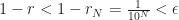 . But all we know of
  has to be smaller than each and every positive number. The biggest number that’s smaller than every positive number is zero. So the difference between 1 and r must be zero and so they must be equal.
  and function
  are equal. That is, that they are less than
  .
.  . It’s got the same deal as
  is equal to
  since adding zero, that is, adding the number
  , can’t change a quantity. And
  . Same reason:
  is zero. So:

 is less than
  ? And that
  is also
  ? Then you’ve shown that
  . With luck, each of these little pieces is something you can prove.
  . You use this trick all the time because if you can also show that
  , then those two have to be equal.
 , and some right boundary,
  , that’s above the x-axis, and below that curve. And there’s just no finding a, you know, answer. Something that looks like (to make up an answer) the area is
  or something normal like that. The one interesting exception is that you can find the area if the left bound is
  and the right bound
  . That’s done by some clever reasoning and changes of variables which is why we see that and only that in freshman calculus. (Oh, and as a side effect we can get the integral between 0 and infinity, because that has to be half of that.)
 and
and  . If you have three functions,
  , you need first derivatives,
  , as well as second derivatives,
  ,
,  , and
, and  . If you have
  functions and here I’ll call them
  , you need
  derivatives,
 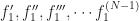 and so on through
  . You see right away this is a fun and exciting thing to calculate. Also why in intro to differential equations you only work this out with two or three functions. Maybe four functions if the class has been really naughty.
 ,
,  , and
, and  are some functions that depend only on the independent variable,
  . Don’t know what they are; don’t care. The differential equation is a lot easier of
 that we want to find, is the same. It’s the right-hand-side that’s different, that’s a constant zero. This is what makes the new equation homogenous. This homogenous equation is easier and we can expect to find two functions,
  and
and  , that solve it. If
  . (The ‘p’ stands for ‘particular’, as in “the solution for this particular
  also has to solve that inhomogenous differential equation. It seems startling but if you work it out, it’s so. (The key is
  also has to solve that inhomogenous differential equation. In fact, for any constants
  and
and  , it has to be that
  is a solution.
 to
to  or maybe
  to
to  . That looks good, but then we have to ask: isn’t that just an operator? Also: then what about differential forms? Or
  is a quadratic form. So is
  ; the x times the y brings this to a second degree. Also a quadratic form is
  . So is
 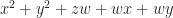 .
.
 . Those of us who don’t do a lot of differential geometry think that looks funny. And we have more familiar ways to write things down. Like, we can put the collection of variables
 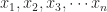 into an ordered
  . If we then think to put the numbers
  into a square
 , and the name “the equation of a circle”.
  is less familiar, but to the crowd reading this, not much less familiar. Fill that out to
  and we have a hyperbola. If we have
  and let that
  then we have an ellipse, something a bit wider than it is tall. Similarly
  is a hyperbola still, just anamorphic.
 just begs to equal
  . Or ellipsoids:
  , set equal to some (positive)
  or
or  , set equal to
  equalling some positive number describes a tube.)
 ? This also wants to be an ellipse.
  , to pick an easy number, is a rotated ellipse. The long axis is along the line described by
  . The short axis is along the line described by
  . How about — let me make this easy.
  ? The equation
  describes a hyperbola, but a rotated one, with the x- and y-axes
  might represent? If you’re thinking “ellipsoid, only it’s at an angle” you’re doing well. It runs really long in one direction, along the plane described by
  can, for sets of integers x, y, z, and w, add up to any positive number you like. (It’s not guaranteed this will happen.
  can’t produce 15.) We know of at least 54 combinations which generate all the positive integers, like
  and
and  and such.
 to mean the sum of all l’s. By mid-November he was integrating functions, and writing out his work as
  . Any mathematics or physics or chemistry or engineering major today would recognize that. A year later he was writing things like
  , which we’d also understand if not quite care to put that way.
 and rewrite it as
  . Leibniz’s notation gives us the idea that taking derivatives is some kind of fraction. It isn’t, but in many problems we act as though it were. It works out often enough we forget that it might not.

 and
and  and many other such exponential functions. One secret of algebra, not appreciated until calculus (or later), is that all these different functions are a single family. Understanding one exponential function lets you understand them all. Mathematicians pick one, the exponential with base e, because we find that convenient.
  .
. 

 but we already have
  in the works here. There is a limit to how many little one-stroke superscripts we need above g. This is the tradeoff to using ‘ for first derivatives. But here’s the important thing:
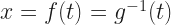


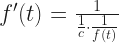


 for the correct value of c. Then all you need do is find a value of ‘c’ that makes that last equation true.
  . What is its velocity? That’s the first derivative of its position, so,
  .
.  is too small to notice. The motion declines into imperceptibility.
  , where
  .
.  , where
  and
and  are some real numbers whose value I don’t care about. What’s important here is that
  .
. 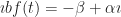 . This is an interesting complex number. Do you see what’s interesting about it? I’ll get there next paragraph.
  and
and  and
and  will all be
  for some real numbers a and b. In this case, you get spirals as t changes. If a is positive, you get points spiralling outward as t increases. If a is negative, you get points spiralling inward toward zero as t increases. If b is positive the spirals go counterclockwise. If b is negative the spirals go clockwise.
  is the same as
  .
.  , is equal to the product of the exponential of those terms. This is a good thing to have in your portfolio. If I remember right, it comes in around the 25th thing. It’s an easy result to have if you already showed something about the logarithms of products.
 is a times the derivative of f plus b times the derivative of g? That’s the differential operator being all linear on us. Similarly, how the integral of
  . And what if we make equations based on doing this

 as if it were a square of
  . It’s not, and
  is not the square of
  . It’s composing
  except to learn some stuff about operators. But you might imagine a world where we did this process all the time. If we did, then we’d develop shorthand for it. Maybe a new operator, call it T, and define it that
  . You see the grammar of treating functions as if they were real numbers becoming familiar. You maybe even noticed the ‘1’ sitting there, serving as the “identity operator”. You know how you’d write out
  if you needed to write it in full.
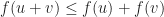 . This is a famous rule, called the triangle inequality. You know how in a triangle, the sum of the lengths of any two legs is greater than the length of the third leg? That’s the rule at work here.
  . This doesn’t have so snappy a name. Sorry. It’s something about being homogeneous, at least.
  then u has to be the additive identity, the vector that works like zero does.
  . Take the absolute value of each of these
  terms. Then … you have choices. You could take those absolute values and add them up. That’s the L1 polynomial norm. Take those absolute values and square them, then add those squares, and take the square root of that sum. That’s the L2 norm. Take the largest absolute value of any of these coefficients. That’s the L∞ norm.
  solves the differential equation. Here I’m going to pretend that the function has one independent variable. Many functions have more than this. Doesn’t matter. Everything I say here extends into two or three or more independent variables. It takes longer and uses more symbols and we don’t need that. The thing about
  going on to however many we need. It can be infinitely many. It certainly is at least up to some
  for some big enough whole number N. These are a set of “
 to represent them. Any function we want is the sum of the coefficient times the matching basis function. That is, there’s some coefficients so that
 and
and  and
and  … well, that’ll take some time, yes. But not forever. Great idea. Is there any way to guarantee that?

 , with some clever scheme that told us for a given k whether it represents a sine or a cosine. It’s less hard work if we have s’s and c’s. And if we have coefficients of both a’s and b’s. That is, we suppose the function
 there, not multiplied by anything more complicated. It makes life easier. It lets us see that the Fourier series for, like, 3 + f(x) is the same as the Fourier series for f(x), except for the leading term. The ½ before that makes easier some work that’s outside the scope of this essay. Accept it as one of the merry, wondrous appearances of ‘2’ in mathematics expressions.
  is true. We can suppose that if we cared we could find what function, or functions, f made that equation true. There is shorthand here. A function has a domain, a range, and a rule. The equation part helps us find the rule. The domain and range we get from the problem. Or we take the implicit rule that both are the biggest sets of real-valued numbers for which the rule parses. Sometimes biggest sets of complex-valued numbers. We get so used to saying “the function” to mean “the rule for the function” that we’ll forget to say that’s what we’re doing.
  ” is continuous. My earlier post lays out what a mathematician means by a “continuous function”. The short version is, we have a good definition for a function being continuous at a point in the domain. If it’s continuous at every point in the domain, it’s a continuous function.
  is a constant function; of course that’s continuous. Your sensible response is to ask if I want a punch in the nose. No, I do not.
 ”. Or, if we become mathematics majors, and we’re in the right courses, we write “
 ”. It’s a format that seems like it’s overcomplicating things. But it’s good at emphasizing the idea that a function can be a map, matching a set in the domain to a set in the range.
  ” we’d be calling for R2. If ‘x’ and ‘z’ both appear, that’s usually a hint that the problem needs coordinates ‘x’, ‘y’, and ‘z’, so that we’d want R3 at least.

 , then, what should we expect it to be for x near zero? It’s irresistible to try out the calculator. Let x be 0.1. 0.01. 0.001. 0.0001. The numbers say this f(x) gets closer and closer to 1. That’s good, right? We know we can’t just put in an x of zero, because there’s some trouble that makes. But we can imagine creeping up on the zero we really wanted. We might spot some obvious prospects for mischief: what if x is negative? We should try -0.1, -0.01, -0.001 and so on. And maybe we won’t get exactly the right answer. But if all we care about is the first (say) three digits and we try out a bunch of x’s and the corresponding f(x)’s agree to those three digits, that’s good enough, right?
  at the origin? You get different results approaching in different directions. And the function doesn’t give obvious signs of imminent danger here.

![Bea: 'Aaaah! I forgot to do my maths homework!' Tonus: 'I did mine.' Bea: 'Can I copy yours?' Tonus: 'Of course you can. I didn't know the answers so I drew a picture of a scary dinosaur.' [ Silent penultimate panel. ] Bea: 'Better than nothing.' Tonus: 'Remember the big teeth. Big teeth make it scary.'](https://nebusresearch.files.wordpress.com/2018/04/anthony-blades_bewley_23-april-2018.gif)
![[ Clown Statistician vs Clown mathematician. ] The Clown Statistician holds up a pie chart, ready to throw it. The mathematician holds up a pi symbol, ready to throw it. Corner squirrel's comment: 'There's always room for more pi.'](https://nebusresearch.files.wordpress.com/2018/04/dave-whamond_reality-check_23-april-2018.gif)
![[ With rain delaying (baseball) practice, Kevin Pelwecki expounds on his new favorite subject --- ] Kevin: 'Launch angle! You want the ball coming off the bat at 25 degrees.' Teammate: 'Anyone else notice we're taking math lessons --- from a guy who barely passed geometry?'](https://nebusresearch.files.wordpress.com/2018/04/neal-rubin-rod-whigham_gil-thorp_24-april-2018.gif)


 . If I have some number called ‘x’ that’s in the domain then I can tell you what number in the domain is matched by the function ‘f’ to ‘x’: it’s the number ‘f(x)’. You were expecting maybe 3.5? I don’t know that about ‘f’, not yet anyway. The one thing I do know about ‘f’, because I insist on it as a condition for appearing, is that it’s continuous. It hasn’t got any jumps, any gaps, any regions where it’s not defined. You could draw a curve representing it with a single, if wriggly, stroke of the pen.


 . That’s my sloppiness, but it’s not uniquely mine. Mathematicians keep this straight by using the symbols


 . The only big difference is that after about the third derivative we give up on adding ‘ marks after the function name ‘f’. It’s just too many little dots. We start writing, like, ‘f(iv)‘ instead. Or if the Roman numerals are too much then ‘f(2038)‘ instead. Or if we don’t want to pin things down to a specific value ‘f(j)‘ with the understanding that ‘j’ is some whole number.
  — then it’s true for the next —
  — is work. But you can get it done.
  . I give you back some other function — say,
  . Then I’m acting as an operator.
  true.
true.  for some ‘v’ that isn’t just zero everywhere.


 and so on. That’s not wrong. The name we give a number doesn’t matter. But it makes it harder to remember what coefficient matches up with, say, x14.)

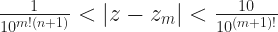
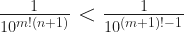
