equilibriums – nebusresearch

Why Stuff Can Orbit, Part 13: To Close A Loop

Why Stuff Can Orbit, featuring a dazed-looking coati (it's a raccoon-like creature from Latin America) and a starry background. — Art courtesy of Thomas K Dye, creator of the web comic **Newshounds**. He has a Patreon for those able to support his work. He’s also open for commissions, starting from US$10.

Previously:

And the supplemental reading:

Today’s is one of the occasional essays in the Why Stuff Can Orbit sequence that just has a lot of equations. I’ve tried not to write everything around equations because I know what they’re like to read. They’re pretty to look at and after about four of them you might as well replace them with a big grey box that reads “just let your eyes glaze over and move down to the words”. It’s even more glaze-y than that for non-mathematicians.

But we do need them. Equations are wonderfully compact, efficient ways to write about things that are true. Especially things that are only true if exacting conditions are met. They’re so good that I’ll often find myself checking a textbook for an explanation of something and looking only at the equations, letting my eyes glaze over the words. That’s a chilling thing to catch yourself doing. Especially when you’ve written some obscure textbooks and a slightly read mathematics blog.

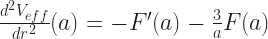
What I had been looking at was a perturbed central-force orbit. We have something, generically called a planet, that orbits the center of the universe. It’s attracted to the center of the universe by some potential energy, which we describe as ‘U(r)’. It’s some number that changes with the distance ‘r’ the planet has from the center of the universe. It usually depends on other stuff too, like some kind of mass of the planet or some constants or stuff. The planet has some angular momentum, which we can call ‘L’ and pretend is a simple number. It’s in truth a complicated number, but we’ve set up the problem where we can ignore the complicated stuff. This angular momentum implies the potential energy allows for a circular orbit at some distance which we’ll call ‘a’ from the center of the universe.

From ‘U(r)’ and ‘L’ we can say whether this is a stable orbit. If it’s stable, a little perturbation, a nudging, from the circular orbit will stay small. If it’s unstable, a little perturbation will keep growing and never stop. If we perturb this circular orbit the planet will wobble back and forth around the circular orbit. Sometimes the radius will be a little smaller than ‘a’, and sometimes it’ll be a little larger than ‘a’. And now I want to see whether we get a stable closed orbit.

The orbit will be closed if the planet ever comes back to the same position and same momentum that it started with. ‘Started’ is a weird idea in this case. But it’s common vocabulary. By it we mean “whatever properties the thing had when we started paying attention to it”. Usually in a problem like this we suppose there’s some measure of time. It’s typically given the name ‘t’ because we don’t want to make this hard on ourselves. The start is some convenient reference time, often ‘t = 0’. That choice usually makes the equations look simplest.

The position of the planet we can describe with two variables. One is the distance from the center of the universe, ‘r’, which we know changes with time: ‘r(t)’. Another is the angle the planet makes with respect to some reference line. The angle we might call ‘θ’ and often do. This will also change in time, then, ‘θ(t)’. We can pick other variables to describe where something is. But they’re going to involve more algebra, more symbol work, than this choice does so who needs it?

Momentum, now, that’s another set of variables we need to worry about. But we don’t need to worry about them. This particular problem is set up so that if we know the position of the planet we also have the momentum. We won’t be able to get both ‘r(t)’ and ‘θ(t)’ back to their starting values without also getting the momentum there. So we don’t have to worry about that. This won’t always work, as see my future series, ‘Why Statistical Mechanics Works’.

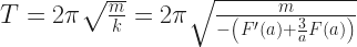
So. We know, because it’s not that hard to work out, how long it takes for ‘r(t)’ to get back to its original, ‘r(0)’, value. It’ll take a time we worked out to be (first big equation here, although we found it a couple essays back):

$T_r = 2\pi\sqrt{ \frac{m}{ -F'(a) - \frac{3}{a} F(a) }}$

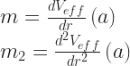
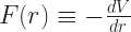
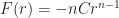
Here ‘m’ is the mass of the planet. And ‘F’ is a useful little auxiliary function. It’s the force that the planet feels when it’s a distance from the origin. It’s defined as $F(r) = -\frac{dU}{dr}$ . It’s convenient to have around. It makes equations like this one simpler, for one. And it’s weird to think of a central force problem where we never, ever see forces. The peculiar thing is we define ‘F’ for every distance the planet might be from the center of the universe. But all we care about is its value at the equilibrium, circular orbit distance of ‘a’. We also care about its first derivative, also evaluated at the distance of ‘a’, which is that $F'(a)$ talk early on in that denominator.

So in the time between time ‘0’ and time ‘T_r‘ the perturbed radius will complete a full loop. It’ll reach its biggest value and its smallest value and get back to the original. (It is so much easier to suppose the perturbation starts at its biggest value at time ‘0’ that we often assume it has. It doesn’t have to be. But if we don’t have something forcing the choice of what time to call ‘0’ on us, why not pick one that’s convenient?) The question is whether ‘θ(t)’ completes a full loop in that time. If it does then we’ve gotten back to the starting position exactly and we have a closed orbit.

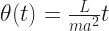
Thing is that the angle will never get back to its starting value. The angle ‘θ(t)’ is always increasing at a rate we call ‘ω’, the angular velocity. This number is constant, at least approximately. Last time we found out what this number was:

$\omega = \frac{L}{ma^2}$

So the angle, over time, is going to look like:

$\theta(t) = \frac{L}{ma^2} t$

And ‘θ(T_r)’ will never equal ‘θ(0)’ again, not unless ‘ω’ is zero. And if ‘ω’ is zero then the planet is racing away from the center of the universe never to be seen again. Or it’s plummeting into the center of the universe to be gobbled up by whatever resides there. In either case, not what we traditionally think of as orbits. Even if we allow these as orbits, these would be nudges too big to call perturbations.

So here’s the resolution. Angles are right awful pains in mathematical physics. This is because increasing an angle by 2π — or decreasing it by 2π — has no visible effect. In the language of the hew-mon, adding 360 degrees to a turn leaves you back where you started. A 45 degree angle is indistinguishable from a 405 degree angle, or a 765 degree angle, or a -315 degree angle, or so on. This makes for all sorts of irritating alternate cases to consider when you try solving for where one thing meets another. But it allows us to have closed orbits.

Because we can have a closed orbit, now, if the radius ‘r(t)’ completes a full oscillation in the time it takes ‘θ(t)’ to grow by 2π. Or to grow by π. Or to grow by ½π. Or a third of π. Or so on.

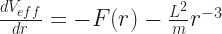
So. Last time we worked out that the angular velocity had to be this number:

$\omega = \frac{L}{ma^2}$

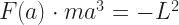
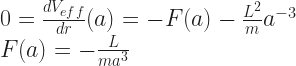
And that looked weird because the central force doesn’t seem to be there. It’s in there. It’s just implicit. We need to know what the central force is to work out what ‘a’ is. But we can make it explicit by using that auxiliary little function ‘F(r)’. In particular, at the circular orbit radius of ‘a’ we have that:

$F(a) = -\frac{L^2}{ma^3}$

I am going to use this to work out what ‘L’ has to be, in terms of ‘F’ and ‘m’ and ‘a’. First, multiply both sides of this equation by ‘ma³‘:

$F(a) \cdot ma^3 = -L^2$

And then both sides by -1:

$-ma^3 F(a) = L^2$

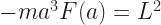
Take the square root — don’t worry, that it will turn out that ‘F(a)’ is a negative number so we’re not doing anything suspicious —

$\sqrt{-ma^3 F(a)} = L$

Now, take that ‘L’ we’ve got and put it back into the equation for angular velocity:

$\omega = \frac{L}{ma^2} = \frac{\sqrt{-ma^3 F(a)}}{ma^2}$

We might look stuck and at what seems like an even worse position. It’s not. When you do enough of these problems you get used to some tricks. For example, that ‘ma²‘ in the denominator we could move under the square root if we liked. This we know because $ma^2 = \sqrt{ \left(ma^2\right)^2 }$ at least as long as ‘ma²‘ is positive. It is.

So. We fall back on the trick of squaring and square-rooting the denominator and so generate this mess:

$\omega = \sqrt{\frac{-ma^3 F(a)}{\left(ma^2\right)^2}} \\ \omega = \sqrt{\frac{-ma^3 F(a)}{m^2 a^4}} \\ \omega = \sqrt{\frac{-F(a)}{ma}}$

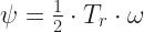
That’s getting nice and simple. Let me go complicate matters. I’ll want to know the angle that the planet sweeps out as the radius goes from its largest to its smallest value. Or vice-versa. This time is going to be half of ‘T_r‘, the time it takes to do a complete oscillation. The oscillation might have started at time ‘t’ of zero, maybe not. But how long it takes will be the same. I’m going to call this angle ‘ψ’, because I’ve written “the angle that the planet sweeps out as the radius goes from its largest to its smallest value” enough times this essay. If ‘ψ’ is equal to π, or one-half π, or one-third π, or some other nice rational multiple of π we’ll get a closed orbit. If it isn’t, we won’t.

So. ‘ψ’ will be one-half times the oscillation time times that angular velocity. This is easy:

$\psi = \frac{1}{2} \cdot T_r \cdot \omega$

Put in the formulas we have for ‘T_r‘ and for ‘ω’. Now it’ll be complicated.

$\psi = \frac{1}{2} 2\pi \sqrt{\frac{m}{-F'(a) - \frac{3}{a} F(a)}} \sqrt{\frac{-F(a)}{ma}}$

Now we’ll make this a little simpler again. We have two square roots of fractions multiplied by each other. That’s the same as the square root of the two fractions multiplied by each other. So we can take numerator times numerator and denominator times denominator, all underneath the square root sign. See if I don’t. Oh yeah and one-half of two π is π but you saw that coming.

$\psi = \pi \sqrt{ \frac{-m F(a)}{-\left(F'(a) + \frac{3}{m}F(a)\right)\cdot ma} }$

OK, so there’s some minus signs in the numerator and denominator worth getting rid of. There’s an ‘m’ in the numerator and the denominator that we can divide out of both sides. There’s an ‘a’ in the denominator that can multiply into a term that has a denominator inside the denominator and you know this would be easier if I could use little cross-out symbols in WordPress LaTeX. If you’re not following all this, try writing it out by hand and seeing what makes sense to cancel out.

$\psi = \pi \sqrt{ \frac{F(a)}{aF'(a) + 3F(a)} }$

This is getting not too bad. Start from a potential energy ‘U(r)’. Use an angular momentum ‘L’ to figure out the circular orbit radius ‘a’. From the potential energy find the force ‘F(r)’. And then, based on what ‘F’ and the first derivative of ‘F’ happen to be, at the radius ‘a’, we can see whether a closed orbit can be there.

I’ve gotten to some pretty abstract territory here. Next time I hope to make things simpler again.

Why Stuff Can Orbit, Part 12: How Fast Is An Orbit?

Previously:

And the supplemental reading:

On to the next piece of looking for stable, closed orbits of a central force. We start from a circular orbit of something around the sun or the mounting point or whatever. The center. I would have saved myself so much foggy writing if I had just decided to make this a sun-and-planet problem. But I had wanted to write the general problem. In this the force attracting the something towards the center has a strength that’s some constant times the distance to the center raised to a power. This is easy to describe in symbols. It’s cluttered to describe in words. This is why symbols are so nice.

The perturbed orbit, the one I want to see close up, looks like an oscillation around that circle. The fact it is a perturbation, a small nudge away from the equilibrium, means how big the perturbation is will oscillate in time. How far the planet (whatever) is from the center will make a sine wave in time. Whether it closes depends on what it does in space.

Part of what it does in space is easy. I just said what the distance from the planet to the center does. But to say where the planet is we need to know how far it is from the center and what angle it makes with respect to some reference direction. That’s a little harder. We also need to know where it is in the third dimension, but that’s so easy. An orbit like this is always in one plane, so we picked that plane to be that of our paper or whiteboard or tablet or whatever we’re using to sketch this out. That’s so easy to answer we don’t even count it as solved.

The angle, though. Here, I mean the angle made by looking at the planet, the center, and some reference direction. This angle can be any real number, although a lot of those angles are going to point to the same direction in space. We’re coming at this from a mathematical view, or a physics view. Or a mathematical physics view. It means we measure this angle as radians instead of degrees. That is, a right angle is $\frac{\pi}{2}$ , not 90 degrees, thank you. A full circle is $2\pi$ and not 360 degrees. We aren’t doing this to be difficult. There are good reasons to use radians. They make the mathematics simpler. What else could matter?

We use $\theta$ as the symbol for this angle. It’s a popular choice. $\theta$ is going to change in time. We’ll want to know how fast it changes over time. This concept we call the angular velocity. For this there are a bunch of different possible notations. The one that I snuck in here two essays ago was ω.

We came at the physics of this orbiting planet from a weird direction. Well, I came at it, and you followed along, and thank you for that. But I never did something like set the planet at a particular distance from the center of the universe and give it a set speed so it would have a circular enough orbit. I set up that we should have some potential energy. That energy implies a central force. It attracts things to the center of the universe. And that there should be some angular momentum that the planet has in its movement. And from that, that there would be some circular orbit. That circular orbit is one with just the right radius and just the right change in angle over time.

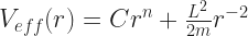
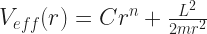
From the potential energy and the angular momentum we can work out the radius of the circular orbit. Suppose your potential energy obeys a rule like $V(r) = Cr^n$ for some number ‘C’ and some power, another number, ‘n’. Suppose your planet has the mass ‘m’. Then you’ll get a circular orbit when the planet’s a distance ‘a’ from the center, if $a^{n + 2} = \frac{L^2}{n C m}$ . And it turns out we can also work out the angular velocity of this circular orbit. It’s all implicit in the amount of angular momentum that the planet has. This is part of why a mathematical physicist looks for concepts like angular momentum. They’re easy to work with, and they yield all sorts of interesting information, given the chance.

I first introduced angular momentum as this number that was how much of something that our something had. It’s got physical meaning, though, reflecting how much … uh … our something would like to keep rotating around the way it has. And this can be written as a formula. The angular momentum ‘L’ is equal to the moment of inertia ‘I’ times the angular velocity ‘ω’. ‘L’ and ‘ω’ are really vectors, and ‘I’ is really a tensor. But we don’t have to worry about this because this kind of problem is easy. We can pretend these are all real numbers and nothing more.

The moment of inertia depends on how the mass of the thing rotating is distributed in space. And it depends on how far the mass is from whatever axis it’s rotating around. For real bodies this can be challenging to work out. It’s almost always a multidimensional integral, haunting students in Calculus III. For a mass in a central force problem, though, it’s easy once again. Please tell me you’re not surprised. If it weren’t easy I’d have some more supplemental reading pieces here first.

For a planet of mass ‘m’ that’s a distance ‘r’ from the axis of rotation, the moment of inertia ‘I’ is equal to ‘mr²‘. I’m fibbing. Slightly. This is for a point mass, that is, something that doesn’t occupy volume. We always look at point masses in this sort of physics. At least when we start. It’s easier, for one thing. And it’s not far off. The Earth’s orbit has a radius just under 150,000,000 kilometers. The difference between the Earth’s actual radius of just over 6,000 kilometers and a point-mass radius of 0 kilometers is a minor correction.

So since we know $L = I\omega$ , and we know $I = mr^2$ , we have $L = mr^2\omega$ and from this:

$\omega = \frac{L}{mr^2}$

We know that ‘r’ changes in time. It oscillates from a maximum to a minimum value like any decent sine wave. So ‘r²‘ is going to oscillate too, like a … sine-squared wave. And then dividing the constant ‘L’ by something oscillating like a sine-squared wave … this implies ω changes in time. So it does. In a possibly complicated and annoying way. So it does. I don’t want to deal with that. So I don’t.

Instead, I am going to summon the great powers of approximation. This perturbed orbit is a tiny change from a circular orbit with radius ‘a’. Tiny. The difference between the actual radius ‘r’ and the circular-orbit radius ‘a’ should be small enough we don’t notice it at first glance. So therefore:

$\omega = \frac{L}{ma^2}$

And this is going to be close enough. You may protest: what if it isn’t? Why can’t the perturbation be so big that ‘a’ is a lousy approximation to ‘r’? To this I say: if the perturbation is that big it’s not a perturbation anymore. It might be an interesting problem. But it’s a different problem from what I’m doing here. It needs different techniques. The Earth’s orbit is different from Halley’s Comet’s orbit in ways we can’t ignore. I hope this answers your complaint. Maybe it doesn’t. I’m on your side there. A lot of mathematical physics, and of analysis, is about making approximations. We need to find perturbations big enough to give interesting results. But not so big they need harder mathematics than you can do. It’s a strange art. I’m not sure I know how to describe how to do it. What I know I’ve learned from doing a lot of problems. You start to learn what kinds of approaches usually pan out.

But what we’re relying on is the same trick we use in analysis. We suppose there is some error margin in the orbit’s radius and angle that’s tolerable. Then if the perturbation means we’d fall outside that error margin, we just look instead at a smaller perturbation. If there is no perturbation small enough to stay within our error margin then the orbit isn’t stable. And we already know it is. Here, we’re looking for closed orbits. People could in good faith argue about whether some particular observed orbit is a small enough perturbation from the circular equilibrium. But they can’t argue about whether there exist some small enough perturbations.

Let me suppose that you’re all right with my answer about big perturbations. There’s at least one more good objection to have here. It’s this: where is the central force? The mass of the planet (or whatever) is there. The angular momentum is there. The equilibrium orbit is there. But where’s the force? Where’s the potential energy we started with? Shouldn’t that appear somewhere in the description of how fast this planet moves around the center?

It should. And it is there, in an implicit form. We get the radius of the circular, equilibrium orbit, ‘a’, from knowing the potential energy. But we’ll do well to tease it out more explicitly. I hope to get there next time.

Why Stuff Can Orbit, Part 11: In Search Of Closure

Previously:

And the supplemental reading:

I’m not ready to finish the series off yet. But I am getting closer to wrapping up perturbed orbits. So I want to say something about what I’m looking for.

In some ways I’m done already. I showed how to set up a central force problem, where some mass gets pulled towards the center of the universe. It can be pulled by a force that follows any rule you like. The rule has to follow some rules. The strength of the pull changes with how far the mass is from the center. It can’t depend on what angle the mass makes with respect to some reference meridian. Once we know how much angular momentum the mass has we can find whether it can have a circular orbit. And we can work out whether that orbit is stable. If the orbit is stable, then for a small nudge, the mass wobbles around that equilibrium circle. It spends some time closer to the center of the universe and some time farther away from it.

I want something a little more, else I can’t carry on this series. I mean, we can make central force problems with more things in them. What we have now is a two-body problem. A three-body problem is more interesting. It’s pretty near impossible to give exact, generally true answers about. We can save things by only looking at very specific cases. Fortunately one is a sun, planet, and moon, where each object is much more massive than the next one. We see a lot of things like that. Four bodies is even more impossible. Things start to clear up if we look at, like, a million bodies, because our idea of what “clear” is changes. I don’t want to do that right now.

Instead I’m going to look for closed orbits. Closed orbits are what normal people would call “orbits”. We’re used to thinking of orbits as, like, satellites going around and around the Earth. We know those go in circles, or ellipses, over and over again. They don’t, but the difference between a closed orbit and what they do is small enough we don’t need to care.

Here, “orbit” means something very close to but not exactly what normal people mean by orbits. Maybe I should have said something about that before. But the difference hasn’t counted for much before.

Start off by thinking of what we need to completely describe what a particular mass is doing. You need to know the central force law that the mass obeys. You need to know, for some reference time, where it is. You also need to know, for that same reference time, what its momentum is. Once you have that, you can predict where it should go for all time to come. You can also work out where it must have been before that reference time. (This we call “retrodicting”. Or “predicting the past”. With this kind of physics problem time has an unnerving symmetry. The tools which forecast what the mass will do in the future are exactly the same as those which tell us what the mass has done in the past.)

Now imagine knowing all the sets of positions and momentums that the mass has had. Don’t look just at the reference time. Look at all the time before the reference time, and look at all the time after the reference time. Imagine highlighting all the sets of positions and momentums the mass ever took on or ever takes on. We highlight them against the universe of all the positions and momentums that the mass could have had if this were a different problem.

What we get is this ribbon-y thread that passes through the universe of every possible setup. This universe of every possible setup we call a “phase space”. It’s easy to explain the “space” part of that name. The phase space obeys the rules we’d expect from a vector space. It also acts in a lot of ways like the regular old space that we live in. The “phase” part I’m less sure how to justify. I suspect we get it because this way of looking at physics problems comes from statistical mechanics. And in that field we’re looking, often, at the different ways a system can behave. This mathematics looks a lot like that of different phases of matter. The changes between solids and liquids and gases are some of what we developed this kind of mathematics to understand, in fact. But this is speculation on my part. I’m not sure why “phase” has attached to this name. I can think of other, harder-to-popularize reasons why the name would make sense too. Maybe it’s the convergence of several reasons. I’d love to hear if someone has a good etymology. If one exists; remember that we still haven’t got the story straight about why ‘m’ stands for the slope of a line.

Anyway, this ribbon of all the arrangements of position and momentum that the mass does ever at any point have we call a “trajectory”. We call it a trajectory because it looks like a trajectory. Sometimes mathematics terms aren’t so complicated. We also call it an “orbit” since very often the problems we like involve trajectories that loop around some interesting area. It looks like a planet orbiting a sun.

A “closed orbit” is an orbit that gets back to where it started. This means you can take some reference time, and wait. Eventually the mass comes back to the same position and the same momentum that you saw at that reference time. This might seem unavoidable. Wouldn’t it have to get back there? And it turns out, no, it doesn’t. A trajectory might wander all over phase space. This doesn’t take much imagination. But even if it doesn’t, if it stays within a bounded region, it could still wander forever without repeating itself. If you’re not sure about that, please consider an old sequence I wrote inspired by the Aardman Animation film Arthur Christmas. Also please consider seeing the Aardman Animation film Arthur Christmas. It is one of the best things this decade has offered us. The short version is, though, that there is a lot of room even in the smallest bit of space. A trajectory is, in a way, a one-dimensional thing that might get all coiled up. But phase space has got plenty of room for that.

And sometimes we will get a closed orbit. The mass can wander around the center of the universe and come back to wherever we first noticed it with the same momentum it first had. A that point it’s locked into doing that same thing again, forever. If it could ever break out of the closed orbit it would have had to the first time around, after all.

Closed orbits, I admit, don’t exist in the real world. Well, the real world is complicated. It has more than a single mass and a single force at work. Energy and momentum are conserved. But we effectively lose both to friction. We call the shortage “entropy”. Never mind. No person has ever seen a circle, and no person ever will. They are still useful things to study. So it is with closed orbits.

An equilibrium orbit, the circular orbit of a mass that’s at exactly the right radius for its angular momentum, is closed. A perturbed orbit, wobbling around the equilibrium, might be closed. It might not. I mean next time to discuss what has to be true to close an orbit.

Why Stuff Can Orbit, Part 10: Where Time Comes From And How It Changes Things

Previously:

And the supplemental reading:

And again my thanks to Thomas K Dye, creator of the web comic Newshounds, for the banner art. He has a Patreon to support his creative habit.

In the last installment I introduced perturbations. These are orbits that are a little off from the circles that make equilibriums. And they introduce something that’s been lurking, unnoticed, in all the work done before. That’s time.

See, how do we know time exists? … Well, we feel it, so, it’s hard for us not to notice time exists. Let me rephrase it then, and put it in contemporary technology terms. Suppose you’re looking at an animated GIF. How do you know it’s started animating? Or that it hasn’t stalled out on some frame?

If the picture changes, then you know. It has to be going. But if it doesn’t change? … Maybe it’s stalled out. Maybe it hasn’t. You don’t know. You know there’s time when you can see change. And that’s one of the little practical insights of physics. You can build an understanding of special relativity by thinking hard about that. Also think about the observation that the speed of light (in vacuum) doesn’t change.

When something physical’s in equilibrium, it isn’t changing. That’s how we found equilibriums to start with. And that means we stop keeping track of time. It’s one more thing to keep track of that doesn’t tell us anything new. Who needs it?

For the planet orbiting a sun, in a perfect circle, or its other little variations, we do still need time. At least some. How far the planet is from the sun doesn’t change, no, but where it is on the orbit will change. We can track where it is by setting some reference point. Where the planet is at the start of our problem. How big is the angle between where the planet is now, the sun (the center of our problem’s universe), and that origin point? That will change over time.

But it’ll change in a boring way. The angle will keep increasing in magnitude at a constant speed. Suppose it takes five time units for the angle to grow from zero degrees to ten degrees. Then it’ll take ten time units for the angle to grow from zero to twenty degrees. It’ll take twenty time units for the angle to grow from zero to forty degrees. Nice to know if you want to know when the planet is going to be at a particular spot, and how long it’ll take to get back to the same spot. At this rate it’ll be eighteen time units before the angle grows to 360 degrees, which looks the same as zero degrees. But it’s not anything interesting happening.

We’ll label this sort of change, where time passes, yeah, but it’s too dull to notice as a “dynamic equilibrium”. There’s change, but it’s so steady and predictable it’s not all that exciting. And I’d set up the circular orbits so that we didn’t even have to notice it. If the radius of the planet’s orbit doesn’t change, then the rate at which its apsidal angle changes, its “angular velocity”, also doesn’t change.

Now, with perturbations, the distance between the planet and the center of the universe will change in time. That was the stuff at the end of the last installment. But also the apsidal angle is going to change. I’ve used ‘r(t)’ to represent the radial distance between the planet and the sun before, and to note that what value it is depends on the time. I need some more symbols.

There’s two popular symbols to use for angles. Both are Greek letters because, I dunno, they’ve always been. (Florian Cajori’s A History of Mathematical Notation doesn’t seem to have anything. And when my default go-to for explaining mathematician’s choices tells me nothing, what can I do? Look at Wikipedia? Sure, but that doesn’t enlighten me either.) One is to use theta, θ. The other is to use phi, φ. Both are good, popular choices, and in three-dimensional problems we’ll often need both. We don’t need both. The orbit of something moving under a central force might be complicated, but it’s going to be in a single plane of movement. The conservation of angular momentum gives us that. It’s not the last thing angular momentum will give us. The orbit might happen not to be in a horizontal plane. But that’s all right. We can tilt our heads until it is.

So I’ll reach deep into the universe of symbols for angles and call on θ for the apsidal angle. θ will change with time, so, ‘θ(t)’ is the angular counterpart to ‘r(t)’.

I’d said before the apsidal angle is the angle made between the planet, the center of the universe, and some reference point. What is my reference point? I dunno. It’s wherever θ(0) is, that is, where the planet is when my time ‘t’ is zero. There’s probably a bootstrapping fallacy here. I’ll cover it up by saying, you know, the reference point doesn’t matter. It’s like the choice of prime meridian. We have to have one, but we can pick whatever one is convenient. So why not pick one that gives us the nice little identity that ‘θ(0) = 0’? If you don’t buy that and insist I pick a reference point first, fine, go ahead. But you know what? The labels on my time axis are arbitrary. There’s no difference in the way physics works whether ‘t’ is ‘0’ or ‘2017’ or ‘21350’. (At least as long as I adjust any time-dependent forces, which there aren’t here.) So we get back to ‘θ(0) = 0’.

For a circular orbit, the dynamic equilibrium case, these are pretty boring, but at least they’re easy to write. They’re:

$r(t) = a \\ \theta(t) = \omega t$

Here ‘a’ is the radius of the circular orbit. And ω is a constant number, the angular velocity. It’s how much a bit of time changes the apsidal angle. And this set of equations is pretty dull. You can see why it barely rates a mention.

The perturbed case gets more interesting. We know how ‘r(t)’ looks. We worked that out last time. It’s some function like:

$r(t) = a + A cos\left(\sqrt{\frac{k}{m}} t\right) + B sin\left(\sqrt{\frac{k}{m}} t\right)$

Here ‘A’ and ‘B’ are some numbers telling us how big the perturbation is, and ‘m’ is the mass of the planet, and ‘k’ is something related to how strong the central force is. And ‘a’ is that radius of the circular orbit, the thing we’re perturbed around.

What about ‘θ(t)’? How’s that look? … We don’t seem to have a lot to go on. We could go back to Newton and all that force equalling the change in momentum over time stuff. We can always do that. It’s tedious, though. We have something better. It’s another gift from the conservation of angular momentum. When we can turn a forces-over-time problem into a conservation-of-something problem we’re usually doing the right thing. The conservation-of-something is typically a lot easier to set up and to track. We’ve used it in the conservation of energy, before, and we’ll use it again. The conservation of ordinary, ‘linear’, momentum helps other problems, though not I’ll grant this one. The conservation of angular momentum will help us here.

So what is angular momentum? … It’s something about ice skaters twirling around and your high school physics teacher sitting on a bar stool spinning a bike wheel. All right. But it’s also a quantity. We can get some idea of it by looking at the formula for calculating linear momentum:

$\vec{p} = m\vec{v}$

The linear momentum of a thing is its inertia times its velocity. This is if the thing isn’t moving fast enough we have to notice relativity. Also if it isn’t, like, an electric or a magnetic field so we have to notice it’s not precisely a thing. Also if it isn’t a massless particle like a photon because see previous sentence. I’m talking about ordinary things like planets and blocks of wood on springs and stuff. The inertia, ‘m’, is rather happily the same thing as its mass. The velocity is how fast something is travelling and which direction it’s going in.

Angular momentum, meanwhile, we calculate with this radically different-looking formula:

$\vec{L} = I\vec{\omega}$

Here, again, talking about stuff that isn’t moving so fast we have to notice relativity. That isn’t electric or magnetic fields. That isn’t massless particles. And so on. Here ‘I’ is the “moment of inertia” and $\vec{w}$ is the angular velocity. The angular velocity is a vector that describes for us how fast the spinning is and what direction the axis around which the thing spins is. The moment of inertia describes how easy or hard it is to make the thing spin around each axis. It’s a tensor because real stuff can be easier to spin in some directions than in others. If you’re not sure that’s actually so, try tossing some stuff in the air so it spins in each of the three major directions. You’ll see.

We’re fortunate. For central force problems the moment of inertia is easy to calculate. We don’t need the tensor stuff. And we don’t even need to notice that the angular velocity is a vector. We know what axis the planet’s rotating around; it’s the one pointing out of the plane of motion. We can focus on the size of the angular velocity, the number ‘ω’. See how they’re different, what with one not having an arrow over the symbol. The arrow-less version is easier. For a planet, or other object, with mass ‘m’ that’s orbiting a distance ‘r’ from the sun, the moment of inertia is:

$I = mr^2$

So we know this number is going to be constant:

$L = mr^2\omega$

The mass ‘m’ doesn’t change. We’re not doing those kinds of problem. So however ‘r’ changes in time, the angular velocity ‘ω’ has to change with it, so that this product stays constant. The angular velocity is how the apsidal angle ‘θ’ changes over time. So since we know ‘L’ doesn’t change, and ‘m’ doesn’t change, then the way ‘r’ changes must tell us something about how ‘θ’ changes. We’ll get into that next time.

Why Stuff Can Orbit, Part 9: How The Spring In The Cosmos Behaves

Previously:

And the supplemental reading:

First, I thank Thomas K Dye for the banner art I have for this feature! Thomas is the creator of the longrunning web comic Newshounds. He’s hoping soon to finish up special editions of some of the strip’s stories and to publish a definitive edition of the comic’s history. He’s also got a Patreon account to support his art habit. Please give his creations some of your time and attention.

Now back to central forces. I’ve run out of obvious fun stuff to say about a mass that’s in a circular orbit around the center of the universe. Before you question my sense of fun, remember that I own multiple pop histories about the containerized cargo industry and last month I read another one that’s changed my mind about some things. These sorts of problems cover a lot of stuff. They cover planets orbiting a sun and blocks of wood connected to springs. That’s about all we do in high school physics anyway. Well, there’s spheres colliding, but there’s no making a central force problem out of those. You can also make some things that look like bad quantum mechanics models out of that. The mathematics is interesting even if the results don’t match anything in the real world.

But I’m sticking with central forces that look like powers. These have potential energy functions with rules that look like V(r) = C rⁿ. So far, ‘n’ can be any real number. It turns out ‘n’ has to be larger than -2 for a circular orbit to be stable, but that’s all right. There are lots of numbers larger than -2. ‘n’ carries the connotation of being an integer, a whole (positive or negative) number. But if we want to let it be any old real number like 0.1 or π or 18 and three-sevenths that’s fine. We make a note of that fact and remember it right up to the point we stop pretending to care about non-integer powers. I estimate that’s like two entries off.

We get a circular orbit by setting the thing that orbits in … a circle. This sounded smarter before I wrote it out like that. Well. We set it moving perpendicular to the “radial direction”, which is the line going from wherever it is straight to the center of the universe. This perpendicular motion means there’s a non-zero angular momentum, which we write as ‘L’ for some reason. For each angular momentum there’s a particular radius that allows for a circular orbit. Which radius? It’s whatever one is a minimum for the effective potential energy:

$V_{eff}(r) = Cr^n + \frac{L^2}{2m}r^{-2}$

This we can find by taking the first derivative of ‘V_eff‘ with respect to ‘r’ and finding where that first derivative is zero. This is standard mathematics stuff, quite routine. We can do with any function whether it represents something physics or not. So:

$\frac{dV_{eff}}{dr} = nCr^{n-1} - 2\frac{L^2}{2m}r^{-3} = 0$

And after some work, this gets us to the circular orbit’s radius:

$r = \left(\frac{L^2}{nCm}\right)^{\frac{1}{n + 2}}$

What I’d like to talk about is if we’re not quite at that radius. If we set the planet (or whatever) a little bit farther from the center of the universe. Or a little closer. Same angular momentum though, so the equilibrium, the circular orbit, should be in the same spot. It happens there isn’t a planet there.

This enters us into the world of perturbations, which is where most of the big money in mathematical physics is. A perturbation is a little nudge away from an equilibrium. What happens in response to the little nudge is interesting stuff. And here we already know, qualitatively, what’s going to happen: the planet is going to rock around the equilibrium. This is because the circular orbit is a stable equilibrium. I’d described that qualitatively last time. So now I want to talk quantitatively about how the perturbation changes given time.

Before I get there I need to introduce another bit of notation. It is so convenient to be able to talk about the radius of the circular orbit that would be the equilibrium. I’d called that ‘r’ up above. But I also need to be able to talk about how far the perturbed planet is from the center of the universe. That’s also really hard not to call ‘r’. Something has to give. Since the radius of the circular orbit is not going to change I’m going to give that a new name. I’ll call it ‘a’. There’s several reasons for this. One is that ‘a’ is commonly used for describing the size of ellipses, which turn up in actual real-world planetary orbits. That’s something we know because this is like the thirteenth part of an essay series about the mathematics of orbits. You aren’t reading this if you haven’t picked up a couple things about orbits on your own. Also we’ve used ‘a’ before, in these sorts of approximations. It was handy in the last supplemental as the point of expansion’s name. So let me make that unmistakable:

$a \equiv r = \left(\frac{L^2}{nCm}\right)^{\frac{1}{n + 2}}$

The $\equiv$ there means “defined to be equal to”. You might ask how this is different from “equals”. It seems like more emphasis to me. Also, there are other names for the circular orbit’s radius that I could have used. ‘r_e‘ would be good enough, as the subscript would suggest “radius of equilibrium”. Or ‘r₀‘ would be another popular choice, the 0 suggesting that this is something of key, central importance and also looking kind of like a circle. (That’s probably coincidence.) I like the ‘a’ better there because I know how easy it is to drop a subscript. If you’re working on a problem for yourself that’s easy to fix, with enough cursing and redoing your notes. On a board in front of class it’s even easier to fix since someone will ask about the lost subscript within three lines. In a post like this? It would be a mess.

So now I’m going to look at possible values of the radius ‘r’ that are close to ‘a’. How close? Close enough that ‘V_eff‘, the effective potential energy, looks like a parabola. If it doesn’t look much like a parabola then I look at values of ‘r’ that are even closer to ‘a’. (Do you see how the game is played? If you don’t, look closer. Yes, this is actually valid.) If ‘r’ is that close to ‘a’, then we can get away with this polynomial expansion:

$V_{eff}(r) \approx V_{eff}(a) + m\cdot(r - a) + \frac{1}{2} m_2 (r - a)^2$

where

$m = \frac{dV_{eff}}{dr}\left(a\right) \\ m_2 = \frac{d^2V_{eff}}{dr^2}\left(a\right)$

The “approximate” there is because this is an approximation. $V_{eff}(r)$ is in truth equal to the thing on the right-hand-side there plus something that isn’t (usually) zero, but that is small.

I am sorry beyond my ability to describe that I didn’t make that ‘m’ and ‘m₂‘ consistent last week. That’s all right. One of these is going to disappear right away.

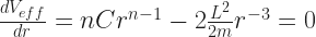
Now, what $V_{eff}(a)$ is? Well, that’s whatever you get from putting in ‘a’ wherever you start out seeing ‘r’ in the expression for $V_{eff}(r)$ . I’m not going to bother with that. Call it math, fine, but that’s just a search-and-replace on the character ‘r’. Also, where I’m going next, it’s going to disappear, never to be seen again, so who cares? What’s important is that this is a constant number. If ‘r’ changes, the value of $V_{eff}(a)$ does not, because ‘r’ doesn’t appear anywhere in $V_{eff}(a)$ .

How about ‘m’? That’s the value of the first derivative of ‘V_eff‘ with respect to ‘r’, evaluated when ‘r’ is equal to ‘a’. That might be something. It’s not, because of what ‘a’ is. It’s the value of ‘r’ which would make $\frac{dV_{eff}}{dr}(r)$ equal to zero. That’s why ‘a’ has that value instead of some other, any other.

So we’ll have a constant part ‘V_eff(a)’, plus a zero part, plus a part that’s a parabola. This is normal, by the way, when we do expansions around an equilibrium. At least it’s common. Good to see it. To find ‘m₂‘ we have to take the second derivative of ‘V_eff(r)’ and then evaluate it when ‘r’ is equal to ‘a’ and ugh but here it is.

$\frac{d^2V_{eff}}{dr^2}(r) = n (n - 1) C r^{n - 2} + 3\cdot\frac{L^2}{m}r^{-4}$

And at the point of approximation, where ‘r’ is equal to ‘a’, it’ll be:

$m_2 = \frac{d^2V_{eff}}{dr^2}(a) = n (n - 1) C a^{n - 2} + 3\cdot\frac{L^2}{m}a^{-4}$

We know exactly what ‘a’ is so we could write that out in a nice big expression. You don’t want to. I don’t want to. It’s a bit of a mess. I mean, it’s not hard, but it has a lot of symbols in it and oh all right. Here. Look fast because I’m going to get rid of that as soon as I can.

$m_2 = \frac{d^2V_{eff}}{dr^2}(a) = n (n - 1) C \left(\frac{L^2}{n C m}\right)^{n - 2} + 3\cdot\frac{L^2}{m}\left(\frac{L^2}{n C m}\right)^{-4}$

For the values of ‘n’ that we actually care about because they turn up in real actual physics problems this expression simplifies some. Enough, anyway. If we pretend we know nothing about ‘n’ besides that it is a number bigger than -2 then … ugh. We don’t have a lot that can clean it up.

Here’s how. I’m going to define an auxiliary little function. Its role is to contain our symbolic sprawl. It has a legitimate role too, though. At least it represents something that it makes sense to give a name. It will be a new function, named ‘F’ and that depends on the radius ‘r’:

$F(r) \equiv -\frac{dV}{dr}$

Notice that’s the derivative of the original ‘V’, not the angular-momentum-equipped ‘V_eff‘. This is the secret of its power. It doesn’t do anything to make $V_{eff}(r)$ easier to work with. It starts being good when we take its derivatives, though:

$\frac{dV_{eff}}{dr} = -F(r) - \frac{L^2}{m}r^{-3}$

That already looks nicer, doesn’t it? It’s going to be really slick when you think about what ‘F(a)’ is. Remember that ‘a’ is the value for ‘r’ which makes the derivative of ‘V_eff‘ equal to zero. So … I may not know much, but I know this:

$0 = \frac{dV_{eff}}{dr}(a) = -F(a) - \frac{L^2}{m}a^{-3} \\ F(a) = -\frac{L}{ma^3}$

I’m not going to say what value F(r) has for other values of ‘r’ because I don’t care. But now look at what it does for the second derivative of ‘V_eff‘:

$\frac{d^2 V_{eff}}{dr^2}(r) = -F'(r) + 3\frac{L^2}{mr^4}$

Here the ‘F'(r)’ is a shorthand way of writing ‘the derivative of F with respect to r’. You can do when there’s only the one free variable to consider. And now something magic that happens when we look at the second derivative of ‘V_eff‘ when ‘r’ is equal to ‘a’ …

$\frac{d^2 V_{eff}}{dr^2}(a) = -F'(a) - \frac{3}{a} F(a)$

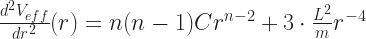
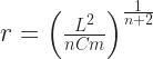
We get away with this because we happen to know that ‘F(a)’ is equal to $-\frac{L}{ma^3}$ and doesn’t that work out great? We’ve turned a symbolic mess into a … less symbolic mess.

Now why do I say it’s legitimate to introduce ‘F(r)’ here? It’s because minus the derivative of the potential energy with respect to the position of something can be something of actual physical interest. It’s the amount of force exerted on the particle by that potential energy at that point. The amount of force on a thing is something that we could imagine being interested in. Indeed, we’d have used that except potential energy is usually so much easier to work with. I’ve avoided it up to this point because it wasn’t giving me anything I needed. Here, I embrace it because it will save me from some awful lines of symbols.

Because with this expression in place I can write the approximation to the potential energy of:

$V_{eff}(r) \approx V_{eff}(a) + \frac{1}{2} \left( -F'(a) - \frac{3}{a}F(a) \right) (r - a)^2$

So if ‘r’ is close to ‘a’, then the polynomial on the right is a good enough approximation to the effective potential energy. And that potential energy has the shape of a spring’s potential energy. We can use what we know about springs to describe its motion. Particularly, we’ll have this be true:

$\frac{dp}{dt} = -\frac{dv_{eff}}{dr}(r) = -\left( F'(a) + \frac{3}{a} F(a)\right) r$

Here, ‘p’ is the (linear) momentum of whatever’s orbiting, which we can treat as equal to ‘mr’, the mass of the orbiting thing times how far it is from the center. You may sense in me some reluctance about doing this, what with that ‘we can treat as equal to’ talk. There’s reasons for this and I’d have to get deep into geometry to explain why. I can get away with specifically this use because the problem allows it. If you’re trying to do your own original physics problem inspired by this thread, and it’s not orbits like this, be warned. This is a spot that could open up to a gigantic danger pit, lined at the bottom with sharp spikes and angry poison-clawed mathematical tigers and I bet it’s raining down there too.

So we can rewrite all this as

$m\frac{d^2r}{dt^2} = -\frac{dv_{eff}}{dr}(r) = -\left( F'(a) + \frac{3}{a} F(a)\right) r$

And when we learned everything interesting there was to know about springs we learned what the solutions to this look like. Oh, in that essay the variable that changed over time was called ‘x’ and here it’s called ‘r’, but that’s not an actual difference. ‘r’ will be some sinusoidal curve:

$r(t) = A cos\left(\sqrt{\frac{k}{m}} t\right) + B sin\left(\sqrt{\frac{k}{m}} t\right)$

where, here, ‘k’ is equal to that whole mass of constants on the right-hand side:

$k = -\left( F'(a) + \frac{3}{a} F(a)\right)$

I don’t know what ‘A’ and ‘B’ are. It’ll depend on just what the perturbation is like, how far the planet is from the circular orbit. But I can tell you what the behavior is like. The planet will wobble back and forth around the circular orbit, sometimes closer to the center, sometimes farther away. It’ll spend as much time closer to the center than the circular orbit as it does farther away. And the period of that oscillation will be

$T = 2\pi\sqrt{\frac{m}{k}} = 2\pi\sqrt{\frac{m}{-\left(F'(a) + \frac{3}{a}F(a)\right)}}$

This tells us something about what the orbit of a thing not in a circular orbit will be like. Yes, I see you in the back there, quivering with excitement about how we’ve got to elliptical orbits. You’re moving too fast. We haven’t got that. There will be elliptical orbits, yes, but only for a very particular power ‘n’ for the potential energy. Not for most of them. We’ll see.

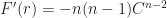
It might strike you there’s something in that square root. We need to take the square root of a positive number, so maybe this will tell us something about what kinds of powers we’re allowed. It’s a good thought. It turns out not to tell us anything useful, though. Suppose we started with $V(r) = Cr^n$ . Then $F(r) = -nCr^{n - 1}$ , and $F'(r) = -n(n - 1)C^{n - 2}$ . Sad to say, this leads us to a journey which reveals that we need ‘n’ to be larger than -2 or else we don’t get oscillations around a circular orbit. We already knew that, though. We already found we needed it to have a stable equilibrium before. We can see there not being a period for these oscillations around the circular orbit as another expression of the circular orbit not being stable. Sad to say, we haven’t got something new out of this.

We will get to new stuff, though. Maybe even ellipses.

How Mathematical Physics Works: Another Course In 2200 Words

OK, I need some more background stuff before returning to the Why Stuff Can Orbit series. Last week I explained how to take derivatives, which is one of the three legs of a Calculus I course. Now I need to say something about why we take derivatives. This essay won’t really qualify you to do mathematical physics, but it’ll at least let you bluff your way through a meeting with one.

We care about derivatives because we’re doing physics a smart way. This involves thinking not about forces but instead potential energy. We have a function, called V or sometimes U, that changes based on where something is. If we need to know the forces on something we can take the derivative, with respect to position, of the potential energy.

The way I’ve set up these central force problems makes it easy to shift between physical intuition and calculus. Draw a scribbly little curve, something going up and down as you like, as long as it doesn’t loop back on itself. Also, don’t take the pen from paper. Also, no corners. That’s just cheating. Smooth curves. That’s your potential energy function. Take any point on this scribbly curve. If you go to the right a little from that point, is the curve going up? Then your function has a positive derivative at that point. Is the curve going down? Then your function has a negative derivative. Find some other point where the curve is going in the other direction. If it was going up to start, find a point where it’s going down. Somewhere in-between there must be a point where the curve isn’t going up or going down. The Intermediate Value Theorem says you’re welcome.

These points where the potential energy isn’t increasing or decreasing are the interesting ones. At least if you’re a mathematical physicist. They’re equilibriums. If whatever might be moving happens to be exactly there, then it’s not going to move. It’ll stay right there. Mathematically: the force is some fixed number times the derivative of the potential energy there. The potential energy’s derivative is zero there. So the force is zero and without a force nothing’s going to change. Physical intuition: imagine you laid out a track with exactly the shape of your curve. Put a marble at this point where the track isn’t rising and isn’t falling. Does the marble move? No, but if you’re not so sure about that read on past the next paragraph.

Mathematical physicists learn to look for these equilibriums. We’re taught to not bother with what will happen if we release this particle at this spot with this velocity. That is, you know, not looking at any particular problem someone might want to know. We look instead at equilibriums because they help us describe all the possible behaviors of a system. Mathematicians are sometimes characterized as lazy in spirit. This is fair. Mathematicians will start out with a problem looking to see if it’s just like some other problem someone already solved. But the flip side is if one is going to go to the trouble of solving a new problem, she’s going to really solve it. We’ll work out not just what happens from some one particular starting condition. We’ll try to describe all the different kinds of thing that could happen, and how to tell which of them does happen for your measly little problem.

If you actually do have a curvy track and put a marble down on its equilibrium it might yet move. Suppose the track is rising a while and then falls back again; putting the marble at top and it’s likely to roll one way or the other. If it doesn’t it’s probably because of friction; the track sticks a little. If it were a really smooth track and the marble perfectly round then it’d fall. Give me this. But even with a perfectly smooth track and perfectly frictionless marble it’ll still roll one way or another. Unless you put it exactly at the spot that’s the top of the hill, not a bit to the left or the right. Good luck.

What’s happening here is the difference between a stable and an unstable equilibrium. This is again something we all have a physical intuition for. Imagine you have something that isn’t moving. Give it a little shove. Does it stay about like it was? Then it’s stable. Does it break? Then it’s unstable. The marble at the top of the track is at an unstable equilibrium; a little nudge and it’ll roll away. If you had a marble at the bottom of a track, inside a valley, then it’s a stable equilibrium. A little nudge will make the marble rock back and forth but it’ll stay nearby.

Yes, if you give it a crazy big whack the marble will go flying off, never to be seen again. We’re talking about small nudges. No, smaller than that. This maybe sounds like question-begging to you. But what makes for an unstable equilibrium is that no nudge is too small. The nudge — perturbation, in the trade — will just keep growing. In a stable equilibrium there’s nudges small enough that they won’t keep growing. They might not shrink, but they won’t grow either.

So how to tell which is which? Well, look at your potential energy and imagine it as a track with a marble again. Where are the unstable equilibriums? They’re the ones at tops of hills. Near them the curve looks like a cup pointing down, to use the metaphor every Calculus I class takes. Where are the stable equilibriums? They’re the ones at bottoms of valleys. Near them the curve looks like a cup pointing up. Again, see Calculus I.

We may be able to tell the difference between these kinds of equilibriums without drawing the potential energy. We can use the second derivative. To find the second derivative of a function you take the derivative of a function and then — you may want to think this one over — take the derivative of that. That is, you take the derivative of the original function a second time. Sometimes higher mathematics gives us terms that aren’t too hard.

So if you have a spot where you know there’s an equilibrium, look at what the second derivative at that spot is. If it’s positive, you have a stable equilibrium. If it’s negative, you have an unstable equilibrium. This is called “Second Derivative Test”, as it was named by a committee that figured it was close enough to 5 pm and why cause trouble?

If the second derivative is zero there, um, we can’t say anything right now. The equilibrium may also be an inflection point. That’s where the growth of something pauses a moment before resuming. Or where the decline of something pauses a moment before resuming. In either case that’s still an unstable equilibrium. But it doesn’t have to be. It could still be a stable equilibrium. It might just have a very smoothly flat base. No telling just from that one piece of information and this is why we have to go on to other work.

But this gets at how we’d like to look at a system. We look for its equilibriums. We figure out which equilibriums are stable and which ones are unstable. With a little more work we can say, if the system starts out like this it’ll stay near that equilibrium. If it starts out like that it’ll stay near this whole other equilibrium. If it starts out this other way, it’ll go flying off to the end of the universe. We can solve every possible problem at once and never have to bother with a particular case. This feels good.

It also gives us a little something more. You maybe have heard of a tangent line. That’s a line that’s, er, tangent to a curve. Again with the not-too-hard terms. What this means is there’s a point, called the “point of tangency”, again named by a committee that wanted to get out early. And the line just touches the original curve at that point, and it’s going in exactly the same direction as the original curve at that point. Typically this means the line just grazes the curve, at least around there. If you’ve ever rolled a pencil until it just touched the edge of your coffee cup or soda can, you’ve set up a tangent line to the curve of your beverage container. You just didn’t think of it as that because you’re not daft. Fair enough.

Mathematicians will use tangents because a tangent line has values that are so easy to calculate. The function describing a tangent line is a polynomial and we llllllllove polynomials, correctly. The tangent line is always easy to understand, however hard the original function was. Its value, at the equilibrium, is exactly what the original function’s was. Its first derivative, at the equilibrium, is exactly what the original function’s was at that point. Its second derivative is zero, which might or might not be true of the original function. We don’t care.

We don’t use tangent lines when we look at equilibriums. This is because in this case they’re boring. If it’s an equilibrium then its tangent line is a horizontal line. No matter what the original function was. It’s trivial: you know the answer before you’ve heard the question.

Ah, but, there is something mathematical physicists do like. The tangent line is boring. Fine. But how about, using the second derivative, building a tangent … well, “parabola” is the proper term. This is a curve that’s a quadratic, that looks like an open bowl. It exactly matches the original function at the equilibrium. Its derivative exactly matches the original function’s derivative at the equilibrium. Its second derivative also exactly matches the original function’s second derivative, though. Third derivative we don’t care about. It’s so not important here I can’t even finish this sentence in a

What this second-derivative-based approximation gives us is a parabola. It will look very much like the original function if we’re close to the equilibrium. And this gives us something great. The great thing is this is the same potential energy shape of a weight on a spring, or anything else that oscillates back and forth. It’s the potential energy for “simple harmonic motion”.

And that’s great. We start studying simple harmonic motion, oh, somewhere in high school physics class because it’s so much fun to play with slinkies and springs and accidentally dropping weights on our lab partners. We never stop. The mathematics behind it is simple. It turns up everywhere. If you understand the mathematics of a mass on a spring you have a tool that relevant to pretty much every problem you ever have. This approximation is part of that. Close to a stable equilibrium, whatever system you’re looking at has the same behavior as a weight on a spring.

It may strike you that a mass on a spring is itself a central force. And now I’m saying that within the central force problem I started out doing, stuff that orbits, there’s another central force problem. This is true. You’ll see that in a few Why Stuff Can Orbit essays.

So far, by the way, I’ve talked entirely about a potential energy with a single variable. This is for a good reason: two or more variables is harder. Well of course it is. But the basic dynamics are still open. There’s equilibriums. They can be stable or unstable. They might have inflection points. There is a new kind of behavior. Mathematicians call it a “saddle point”. This is where in one direction the potential energy makes it look like a stable equilibrium while in another direction the potential energy makes it look unstable. Examples of it kind of look like the shape of a saddle, if you haven’t looked at an actual saddle recently. (If you really want to know, get your computer to plot the function z = x² – y² and look at the origin, where x = 0 and y = 0.) Well, there’s points on an actual saddle that would be saddle points to a mathematician. It’s unstable, because there’s that direction where it’s definitely unstable.

So everything about multivariable functions is longer, and a couple bits of it are harder. There’s more chances for weird stuff to happen. I think I can get through most of Why Stuff Can Orbit without having to know that. But do some reading up on that before you take a job as a mathematical physicist.

Why Stuff Can Orbit, Part 5: Why Physics Doesn’t Work And What To Do About It

Less way previously:

My title’s hyperbole, to the extent it isn’t clickbait. Of course physics works. By “work” I mean “model the physical world in useful ways”. If it didn’t work then we would call it “pure” mathematics instead. Mathematicians would study it for its beauty. Physicists would be left to fend for themselves. “Useful” I’ll say means “gives us something interesting to know”. “Interesting” I’ll say if you want to ask what that means then I think you’re stalling.

But what I mean is that Newtonian physics, the physics learned in high school, doesn’t work. Well, it works, in that if you set up a problem right and calculate right you get answers that are right. It’s just not efficient, for a lot of interesting problems. Don’t ask me about interesting again. I’ll just say the central-force problems from this series are interesting.

Newtonian, high school type, physics works fine. It shines when you have only a few things to keep track of. In this central force problem we have one object, a planet-or-something, that moves. And only one force, one that attracts the planet to or repels the planet from the center, the Origin. This is where we’d put the sun, in a planet-and-sun system. So that seems all right as far as things go.

It’s less good, though, if there’s constraints. If it’s not possible for the particle to move in any old direction, say. That doesn’t turn up here; we can imagine a planet heading in any direction relative to the sun. But it’s also less good if there’s a symmetry in what we’re studying. And in this case there is. The strength of the central force only changes based on how far the planet is from the origin. The direction only changes based on what direction the planet is relative to the origin. It’s a bit daft to bother with x’s and y’s and maybe even z’s when all we care about is the distance from the origin. That’s a number we’ve called ‘r’.

So this brings us to Lagrangian mechanics. This was developed in the 18th century by Joseph-Louis Lagrange. He’s another of those 18th century mathematicians-and-physicists with his name all over everything. Lagrangian mechanics are really, really good when there’s a couple variables that describe both what we’d like to observe about the system and its energy. That’s exactly what we have with central forces. Give me a central force, one that’s pointing directly toward or away from the origin, and that grows or shrinks as the radius changes. I can give you a potential energy function, V(r), that matches that force. Give me an angular momentum L for the planet to have, and I can give you an effective potential energy function, V_eff(r). And that effective potential energy lets us describe how the coordinates change in time.

The method looks roundabout. It depends on two things. One is the coordinate you’re interested in, in this case, r. The other is how fast that coordinate changes in time. This we have a couple of ways of denoting. When working stuff out on paper that’s often done by putting a little dot above the letter. If you’re typing, dots-above-the-symbol are hard. So we mark it as a prime instead: r’. This works well until the web browser or the word processor assumes we want smart quotes and we already had the r’ in quote marks. At that point all hope of meaning is lost and we return to communicating by beating rocks with sticks. We live in an imperfect world.

What we get out of this is a setup that tells us how fast r’, how fast the coordinate we’re interested in changes in time, itself changes in time. If the coordinate we’re interested in is the ordinary old position of something, then this describes the rate of change of the velocity. In ordinary English we call that the acceleration. What makes this worthwhile is that the coordinate doesn’t have to be the position. It also doesn’t have to be all the information we need to describe the position. For the central force problem r here is just how far the planet is from the center. That tells us something about its position, but not everything. We don’t care about anything except how far the planet is from the center, not yet. So it’s fine we have a setup that doesn’t tell us about the stuff we don’t care about.

How fast r’ changes in time will be proportional to how fast the effective potential energy, V_eff(r), changes with its coordinate. I so want to write “changes with position”, since these coordinates are usually the position. But they can be proxies for the position, or things only loosely related to the position. For an example that isn’t a central force, think about a spinning top. It spins, it wobbles, it might even dance across the table because don’t they all do that? The coordinates that most sensibly describe how it moves are about its rotation, though. What axes is it rotating around? How do those change in time? Those don’t have anything particular to do with where the top is. That’s all right. The mathematics works just fine.

A circular orbit is one where the radius doesn’t change in time. (I’ll look at non-circular orbits later on.) That is, the radius is not increasing and is not decreasing. If it isn’t getting bigger and it isn’t getting smaller, then it’s got to be staying the same. Not all higher mathematics is tricky. The radius of the orbit is the thing I’ve been calling r all this time. So this means that r’, how fast r is changing with time, has to be zero. Now a slightly tricky part.

How fast is r’, the rate at which r changes, changing? Well, r’ never changes. It’s always the same value. Anytime something is always the same value the rate of its change is zero. This sounds tricky. The tricky part is that it isn’t tricky. It’s coincidental that r’ is zero and the rate of change of r’ is zero, though. If r’ were any fixed, never-changing number, then the rate of change of r’ would be zero. It happens that we’re interested in times when r’ is zero.

So we’ll find circular orbits where the change in the effective potential energy, as r changes, is zero. There’s an easy-to-understand intuitive idea of where to find these points. Look at a plot of Veff and imagine this is a smooth track or the cross-section of a bowl or the landscaping of a hill. Imagine dropping a ball or a marble or a bearing or something small enough to roll in it. Where does it roll to a stop? That’s where the change is zero.

It’s too much bother to make a bowl or landscape a hill or whatnot for every problem we’re interested in. We might do it anyway. Mathematicians used to, to study problems that were too complicated to do by useful estimates. These were “analog computers”. They were big in the days before digital computers made it no big deal to simulate even complicated systems. We still need “analog computers” or models sometimes. That’s usually for problems that involve chaotic stuff like turbulent fluids. We call this stuff “wind tunnels” and the like. It’s all a matter of solving equations by building stuff.

We’re not working with problems that complicated. There isn’t the sort of chaos lurking in this problem that drives us to real-world stuff. We can find these equilibriums by working just with symbols instead.

Why Stuff Can Orbit, Part 4: On The L

Less way previously:

We were chatting about central forces. In these a small object — a satellite, a planet, a weight on a spring — is attracted to the center of the universe, called the origin. We’ve been studying this by looking at potential energy, a function that in this case depends only on how far the object is from the origin. But to find circular orbits, we can’t just look at the potential energy. We have to modify this potential energy to account for angular momentum. This essay I mean to discuss that angular momentum some.

Let me talk first about the potential energy. Mathematical physicists usually write this as a function named U or V. I’m using V. That’s what my professor used teaching this, back when I was an undergraduate several hundred thousand years ago. A central force, by definition, changes only with how far you are from the center. I’ve put the center at the origin, because I am not a madman. This lets me write the potential energy as V = V(r).

V(r) could, in principle, be anything. In practice, though, I am going to want it to be r raised to a power. That is, V(r) is equal to C rⁿ. The ‘C’ here is a constant. It’s a scaling constant. The bigger a number it is the stronger the central force. The closer the number is to zero the weaker the force is. In standard units, gravity has a constant incredibly close to zero. This makes orbits very big things, which generally works out well for planets. In the mathematics of masses on springs, the constant is closer to middling little numbers like 1.

The ‘n’ here is a deceiver. It’s a constant number, yes, and it can be anything we want. But the use of ‘n’ as a symbol has connotations. Usually when a mathematician or a physicist writes ‘n’ it’s because she needs a whole number. Usually a positive whole number. Sometimes it’s negative. But we have a legitimate central force if ‘n’ is any real number: 2, -1, one-half, the square root of π, any of that is good. If you just write ‘n’ without explanation, the reader will probably think “integers”, possibly “counting numbers”. So it’s worth making explicit when this isn’t so. It’s bad form to surprise the reader with what kind of number you’re even talking about.

(Some number of essays on we’ll find out that the only values ‘n’ can have that are worth anything are -1, 2, and 7. And 7 isn’t all that good. But we aren’t supposed to know that yet.)

C rⁿ isn’t the only kind of central force that could exist. Any function rule would do. But it’s enough. If we wanted a more complicated rule we could just add two, or three, or more potential energies together. This would give us $V(r) = C_1 r^{n_1} + C_2 r^{n_2}$ , with C₁ and C₂ two possibly different numbers, and n₁ and n₂ two definitely different numbers. (If n₁ and n₂ were the same number then we should just add C₁ and C₂ together and stop using a more complicated expression than we need.) Remember that Newton’s Law of Motion about the sum of multiple forces being something vector something something direction? When we look at forces as potential energy functions, that law turns into just adding potential energies together. They’re well-behaved that way.

And if we can add these r-to-a-power potential energies together then we’ve got everything we need. Why? Polynomials. We can approximate most any potential energy that would actually happen with a big enough polynomial. Or at least a polynomial-like function. These r-to-a-power forces are a basis set for all the potential energies we’re likely to care about. Understand how to work with one and you understand how to work with them all.

Well, one exception. The logarithmic potential, V(r) = C log(r), is really interesting. And it has real-world applicability. It describes how strongly two vortices, two whirlpools, attract each other. You can write the logarithm as a polynomial. But logarithms are pretty well-behaved functions. You might be better off just doing that as a special case.

Still, at least to start with, we’ll stick with V(r) = C rⁿ and you know what I mean by all those letters now. So I’m free to talk about angular momentum.

You’ve probably heard of momentum. It’s got something to do with movement, only sports teams and political campaigns are always gaining or losing it somehow. When we talk of that we’re talking of linear momentum. It describes how much mass is moving how fast in what direction. So it’s a vector, in three-dimensional space. Or two-dimensional space if you’re making the calculations easier. To find what the vector is, we make a list of every object that’s moving. We take its velocity — how fast it’s moving and in what direction — and multiply that by its mass. Mass is a single number, a scalar, and we’re always allowed to multiply a vector by a scalar. This gets us another vector. Once we’ve done that for everything that’s moving, we add all those product vectors together. We can always add vectors together. And this gives us a grand total vector, the linear momentum of the system.

And that’s conserved. If one part of the system starts moving slower it’s because other parts are moving faster, and vice-versa. In the real world momentum seems to evaporate. That’s because some of the stuff moving faster turns out to be air objects bumped into, or particles of the floor that get dragged along by friction, or other stuff we don’t care about. That momentum can seem to evaporate is what makes its use in talking about ports teams or political campaigns make sense. It also annoys people who want you to know they understand science words better than you. So please consider this my authorization to use “gaining” and “losing” momentum in this sense. Ignore complainers. They’re the people who complain the word “decimate” gets used to mean “destroy way more than ten percent of something”, even though that’s the least bad mutation of an English word’s meaning in three centuries.

Angular momentum is also a vector. It’s also conserved. We can calculate what that vector is by the same sort of process, that of calculating something on each object that’s spinning and adding it all up. In real applications it can seem to evaporate. But that’s also because the angular momentum is going into particles of air. Or it rubs off grease on the axle. Or it does other stuff we wish we didn’t have to deal with.

The calculation is a little harder to deal with. There’s three parts to a spinning thing. There’s the thing, and there’s how far it is from the axis it’s spinning around, and there’s how fast it’s spinning. So you need to know how fast it’s travelling in the direction perpendicular to the shortest line between the thing and the axis it’s spinning around. Its angular momentum is going to be as big as the mass times the distance from the axis times the perpendicular speed. It’s going to be pointing in whichever axis direction makes its movement counterclockwise. (Because that’s how physicists started working this out and it would be too much bother to change now.)

You might ask: wait, what about stuff like a wheel that’s spinning around its center? Or a ball being spun? That can’t be an angular momentum of zero? How do we work that out? The answer is: calculus. Also, we don’t need that. This central force problem I’ve framed so that we barely even need algebra for it.

See, we only have a single object that’s moving. That’s the planet or satellite or weight or whatever it is. It’s got some mass, the value of which we call ‘m’ because why make it any harder on ourselves. And it’s spinning around the origin. We’ve been using ‘r’ to mean the number describing how far it is from the origin. That’s the distance to the axis it’s spinning around. Its velocity — well, we don’t have any symbols to describe what that is yet. But you can imagine working that out. Or you trust that I have some clever mathematical-physics tool ready to introduce to work it out. I have, kind of. I’m going to ignore it altogether. For now.

The symbol we use for the total angular momentum in a system is $\vec{L}$ . The little arrow above the symbol is one way to denote “this is a vector”. It’s a good scheme, what with arrows making people think of vectors and it being easy to write on a whiteboard. In books, sometimes, we make do just by putting the letter in boldface, L, which is easier for old-fashioned word processors to do. If we’re sure that the reader isn’t going to forget that L is this vector then we might stop highlighting the fact altogether. That’s even less work to do.

It’s going to be less work yet. Central force problems like this mean the object can move only in a two-dimensional plane. (If it didn’t, it wouldn’t conserve angular momentum: the direction of $\vec{L}$ would have to change. Sounds like magic, but trust me.) The angular momentum’s direction has to be perpendicular to that plane. If the object is spinning around on a sheet of paper, the angular momentum is pointing straight outward from the sheet of paper. It’s pointing toward you if the object is moving counterclockwise. It’s pointing away from you if the object is moving clockwise. What direction it’s pointing is locked in.

All we need to know is how big this angular momentum vector is, and whether it’s positive or negative. So we just care about this number. We can call it ‘L’, no arrow, no boldface, no nothing. It’s just a number, the same as is the mass ‘m’ or distance from the origin ‘r’ or any of our other variables.

If ‘L’ is zero, this means there’s no total angular momentum. This means the object can be moving directly out from the origin, or directly in. This is the only way that something can crash into the center. So if setting L to be zero doesn’t allow that then we know we did something wrong, somewhere. If ‘L’ isn’t zero, then the object can’t crash into the center. If it did we’d be losing angular momentum. The object’s mass times its distance from the center times its perpendicular speed would have to be some non-zero number, even when the distance was zero. We know better than to look for that.

You maybe wonder why we use ‘L’ of all letters for the angular momentum. I do. I don’t know. I haven’t found any sources that say why this letter. Linear momentum, which we represent with $\vec{p}$ , I know. Or, well, I know the story every physicist says about it. p is the designated letter for linear momentum because we used to use the word “impetus”, as in “impulse”, to mean what we mean by momentum these days. And “p” is the first letter in “impetus” that isn’t needed for some more urgent purpose. (“m” is too good a fit for mass. “i” has to work both as an index and as that number which, squared, gives us -1. And for that matter, “e” we need for that exponentials stuff, and “t” is too good a fit for time.) That said, while everybody, everybody, repeats this, I don’t know the source. Perhaps it is true. I can imagine, say, Euler or Lagrange in their writing settling on “p” for momentum and everybody copying them. I just haven’t seen a primary citation showing this is so.

(I don’t mean to sound too unnecessarily suspicious. But just because everyone agrees on the impetus-thus-p story doesn’t mean it’s so. I mean, every Star Trek fan or space historian will tell you that the first space shuttle would have been named Constitution until the Trekkies wrote in and got it renamed Enterprise. But the actual primary documentation that the shuttle would have been named Constitution is weak to nonexistent. I’ve come to the conclusion NASA had no plan in mind to name space shuttles until the Trekkies wrote in and got one named. I’ve done less poking around the impetus-thus-p story, in that I’ve really done none, but I do want it on record that I would like more proof.)

Anyway, “p” for momentum is well-established. So I would guess that when mathematical physicists needed a symbol for angular momentum they looked for letters close to “p”. When you get into more advanced corners of physics “q” gets called on to be position a lot. (Momentum and position, it turns out, are nearly-identical-twins mathematically. So making their symbols p and q offers aesthetic charm. Also great danger if you make one little slip with the pen.) “r” is called on for “radius” a lot. Looking on, “t” is going to be time.

On the other side of the alphabet, well, “o” is just inviting danger. “n” we need to count stuff. “m” is mass or we’re crazy. “l” might have just been the nearest we could get to “p” without intruding on a more urgently-needed symbol. (“s” we use a lot for parameters like length of an arc that work kind of like time but aren’t time.) And then shift to the capital letter, I expect, because a lowercase l looks like a “1”, to everybody’s certain doom.

The modified potential energy, then, is going to include the angular momentum L. At least, the amount of angular momentum. It’s also going to include the mass of the object moving, and the radius r that says how far the object is from the center. It will be:

$V_{eff}(r) = V(r) + \frac{L^2}{2 m r^2}$

V(r) was the original potential, whatever that was. The modifying term, with this square of the angular momentum and all that, I kind of hope you’ll just accept on my word. The L² means that whether the angular momentum is positive or negative, the potential will grow very large as the radius gets small. If it didn’t, there might not be orbits at all. And if the angular momentum is zero, then the effective potential is the same original potential that let stuff crash into the center.

For the sort of r-to-a-power potentials I’ve been looking at, I get an effective potential of:

$V_{eff}(r) = C r^n + \frac{L^2}{2 m r^2}$

where n might be an integer. I’m going to pretend a while longer that it might not be, though. C is certainly some number, maybe positive, maybe negative.

If you pick some values for C, n, L, and m you can sketch this out. If you just want a feel for how this V_eff looks it doesn’t much matter what values you pick. Changing values just changes the scale, that is, where a circular orbit might happen. It doesn’t change whether it happens. Picking some arbitrary numbers is a good way to get a feel for how this sort of problem works. It’s good practice.

Sketching will convince you there are energy minimums, where we can get circular orbits. It won’t say where to find them without some trial-and-error or building a model of this energy and seeing where a ball bearing dropped into it rolls to a stop. We can do this more efficiently.

Why Stuff Can Orbit, Part 3: It Turns Out Spinning Matters

Way previously:

Before the big distractions of Theorem Thursdays and competitive pinball events and all that I was writing up the mathematics of orbits. Last time I’d got to establishing that there can’t be such a thing as an orbit. This seems to disagree with what a lot of people say we can observe. So I want to resolve that problem. Yes, I’m aware I’m posting this on a Thursday, which I said I wasn’t going to do because it’s too hard on me to write. I don’t know how it worked out like that.

Let me get folks who didn’t read the previous stuff up to speed. I’m using as model two things orbiting each other. I’m going to call it a sun and a planet because it’s way too confusing not to give things names. But they don’t have to be a sun and a planet. They can be a planet and moon. They can be a proton and an electron if you want to pretend quantum mechanics isn’t a thing. They can be a wood joist and a block of rubber connected to it by a spring. That’s a legitimate central force. They can even be stuff with completely made-up names representing made-up forces. So far I’m supposing the things are attracted or repelled by a force with a strength that depends on how far they are from each other but on nothing else.

Also I’m supposing there are only two things in the universe. This is because the mathematics of two things with this kind of force is easy to do. An undergraduate mathematics or physics major can do it. The mathematics of three things is too complicated to do. I suppose somewhere around two-and-a-third things the mathematics hard enough you need an expert but the expert can do it.

Mathematicians and physicists will call this sort of problem a “central force” problem. We can make it easier by supposing the sun is at the center of the universe, or at least our coordinate system. So we don’t have to worry about it moving. It’s just there at the center, the “origin”, and it’s only the planet that moves.

Forces are tedious things to deal with. They’re vectors. In this context that makes them bundles of three quantities each related to the other two. We can avoid a lot of hassle by looking at potential energy instead. Potential energy is a scalar, a single number. Numbers are nice and easy. Calculus tells us how to go from potential energy to forces, in case we need the forces. It also tells us how to go from forces to potential energy, so we can do the easier problem instead. So we do.

To write about potential energy mathematical physicists use exactly the letter you would guess they’d use if every other letter were unavailable for some reason: V. Or U, if they prefer. I’ll stick with V. Right now I don’t want to say anything about what rule determines the values of V. I just want to allow that its value changes as the planet’s distance from the star — the radius ‘r’ of its orbit — changes. So we make that clear by writing the potential energy is V = V(r). (The potential energy might change with the mass of the planet or sun, or the strength of gravity in the universe, or whatever. But we’re going to pretend those don’t change, not for the problem we’re doing, so we don’t have to write them out.)

If you draw V(r) versus r you can discover right away circular orbits. They’re ones that are local maximums or local minimums of V(r). Physical intuition will help us here. Imagine the graph of the potential energy as if it were a smooth bowl. Drop a marble into it. Where would the marble come to rest? That’s a local minimum. The radius of that minimum is a circular orbit. (Oh, a local maximum, where the marble is at the top of a hill and doesn’t fall to either side, could be a circular orbit. But it isn’t going to be stable. The marble will roll one way or another given the slightest chance.)

The potential energy for a force like gravity or electric attraction looks like the distance, r, raised to a power. And then multiplied by some number, which is where we hide gravitational constants and masses and all that stuff. Generally, it looks like V(r) = C rⁿ where C is some number and n is some other number. For gravity and electricity that number is -1. For two particles connected by a spring that number n is +2. Could be anything.

The trouble is if you draw these curves you realize that a marble dropped in would never come to a stop. It would roll down to the center, the planet falling into the sun. Or it would roll away forever, the planet racing into deep space. Either way it doesn’t orbit or do anything near orbiting. This seems wrong.

It’s not, though. Suppose the force is repelling, that is, the potential energy gets to be smaller and smaller numbers as the distance increases. Then the two things do race away from each other. Physics students are asked to imagine two positive charges let loose next to each other. Physics students understand they’ll go racing away from each other, even though we don’t see stuff in the real world that does that very often. We suppose the students understand, though. These days I guess you can make an animation of it and people will accept that as if it’s proof of anything.

Suppose the force is attracting. Imagine just dropping a planet out somewhere by a sun. Set it carefully just in place and let it go and get out of the way before happens. This is what we do in physics and mathematics classes, so that’s the kind of fun stuff you skipped if you majored in something else. But then we go on to make calculations about it. But that’ll orbit, right? It won’t just drop down into the sun and get melted or something?

Not so, the way I worded it. If we set the planet into space so it was holding still, not moving at all, then it will fall. Plummet, really. The planet’s attracted to the sun, and it moves in that direction, and it’s just going to keep moving that way. If it were as far from the center as the Earth is from the Sun it’ll take its time, yes, but it’ll fall into the sun and not do anything remotely like orbiting. And yet there’s still orbits. What’s wrong?

What’s wrong is a planet isn’t just sitting still there waiting to fall into the sun. Duh, you say. But why isn’t it just sitting still? That’s because it’s moving. Might be moving in any direction. We can divide that movement up into two pieces. One is the radial movement, how fast it’s moving towards or away from the center, that is, along the radius between sun and planet. If it’s a circular orbit this speed is zero; the planet isn’t moving any closer or farther away. If this speed isn’t zero it might affect how fast the planet falls into the sun, but it won’t affect the fact of whether it does or not. No more than how fast you toss a ball up inside a room changes whether it’ll eventually hit the floor. </p.

It’s the other part, the transverse velocity, that matters. This is the speed the thing is moving perpendicular to the radius. It’s possible that this is exactly zero and then the planet does drop into the sun. It’s probably not. And what that means is that the planet-and-sun system has an angular momentum. Angular momentum is like regular old momentum, only for spinning. And as with regular momentum, the total is conserved. It won’t change over time. When I was growing up this was always illustrated by thinking of ice skaters doing a spin. They pull their arms in, they spin faster. They put their arms out, they spin slower.

(Ice skaters eventually slow down, yes. That’s for the same reasons they slow down if they skate in a straight line even though regular old momentum, called “linear momentum” if you want to be perfectly clear, is also conserved. It’s because they have to get on to the rest of their routine.)

The same thing has to happen with planets orbiting a sun. If the planet moves closer to the sun, it speeds up; if it moves farther away, it slows down. To fall into the exact center while conserving angular momentum demands the planet get infinitely fast. This they don’t typically do.

There was a tipoff to this. It’s from knowing the potential energy V(r) only depends on the distance between sun and planet. If you imagine taking the system and rotating it all by any angle, you wouldn’t get any change in the forces or the way things move. It would just change the values of the coordinates you used to describe this. Mathematical physicists describe this as being “invariant”, which means what you’d imagine, under a “continuous symmetry”, which means a change that isn’t … you know, discontinuous. Rotating thing as if they were on a pivot, that is, instead of (like) reflecting them through a mirror.

And invariance under a continuous symmetry like this leads to a conservation law. This is known from Noether’s Theorem. You can find explained quite well on every pop-mathematics and pop-physics blog ever. It’s a great subject for pop-mathematics/physics writing. The idea, that the geometry of a problem tells us something about its physics and vice-versa, is important. It’s a heady thought without being so exotic as to seem counter-intuitive. And its discoverer was Dr Amalie Emmy Noether. She’s an early-20th-century demonstration of the first-class work that one can expect women to do when they’re not driven out of mathematics. You see why the topic is so near irresistible.

So we have to respect the conservation of angular momentum. This might sound like we have to give up on treating circular orbits as one-variable problems. We don’t have to just yet. We will, eventually, want to look at not just how far the planet is from the origin but also in what direction it is. We don’t need to do that yet. We have a brilliant hack.

We can represent the conservation of angular momentum as a slight repulsive force. It’s not very big if the angular momentum is small. It’s not going to be a very big force unless the planet gets close to the origin, that is, until r gets close to zero. But it does grow large and acts as if the planet is being pushed away. We consider that a pseudoforce. It appears because our choice of coordinates would otherwise miss some important physics. And that’s fine. It’s not wrong any more than, say, a hacksaw is the wrong tool to cut through PVC pipe just because you also need a vise.

This pseudoforce can be paired with a pseduo-potential energy. One of the great things about the potential-energy view of physics is that adding two forces together is as easy as adding their potential energies together. We call the sum of the original potential energy and the angular-momentum-created pseudopotential the “effective potential energy”. Far from the origin, for large radiuses r, this will be almost identical to the original potential energy. Close to the origin, this will be a function that rises up steeply. And as a result there can suddenly be a local minimum. There can be a circular orbit.

Spring potential, which is a parabola growing with the distance r from the origin. And the effective potential, which grows to a vertical asymptote where the radius is zero. — Figure 1. The potential energy of a spring — the red line — and the effective potential energy — the blue line — when the angular momentum is added as a pseudoforce. Without angular momentum in consideration the only equilibrium is at the origin. With angular momentum there’s some circular orbit, somewhere. Don’t pay attention to the numbers on the axes. They don’t mean anything.

Gravitational potential, with a vertical asymptote at the radius equalling zero going down to negative infinitely great numbers and a horizontal asymptote at the radius going off to infinity. And the effective potential, with the vertical asymptote at radius of zero going to positive infinitely great numbers, forcing there to be some minimum: a circular orbit. — Figure 2. The potential energy of a gravitational attraction — the red line — and the effective potential energy — the blue line — when the angular momentum is added as a pseudoforce. Without angular momentum in consideration there’s no equilibrium. The thing, a planet, falls into the center, the sun. With angular momentum there’s some circular orbit. As before the values of the numbers don’t matter and you should just ignore them.

The location of the minimum — the radius of the circular orbit — will depend on the original potential, of course. It’ll also depend on the angular momentum. The smaller the angular momentum the closer to the origin will be the circular orbit. If the angular momentum is zero we have the original potential and the planet dropping into the center again. If the angular momentum is large enough there might not even be a minimum anymore. That matches systems where the planet has escape velocity and can go plunging off into deep space. And we can see this by looking at the plot of the effective velocity even before we calculate things.

This only goes so far as demonstrating a circular orbit should exist. Or giving some conditions for which a circular orbit wouldn’t. We might want to know something more, like where that circular orbit is. Or if it’s possible for there to be an elliptic orbit. Or other shapes. I imagine it’s possible to work this out with careful enough drawings. But at some point it gets easier to just calculate things. We’ll get to that point soon.

Why Stuff Can Orbit, Part 2: Why Stuff Can’t Orbit

Previously:

Laying some groundwork.

As I threatened last week, I want to talk some about central forces. They’re forces in which one particle attracts another with a force that depends only on how far apart the two are. Last week’s essay described some of the assumptions behind the model.

Mostly, we can study two particles interacting as if it were one particle hovering around the origin. The origin is some central reference point. If we’re looking for a circular orbit then we only have to worry about one variable. This would be ‘r’, the radius of the orbit: how far the planet is from the sun it orbits.

Now, central forces can follow any rule you like. Not in reality, of course. In reality there’s two central forces you ever see. One is gravity (electric attraction or repulsion follows the same rule) and the other is springs. But we can imagine there being others. At the end of this string of essays I hope to show why there’s special things about these gravity and spring-type forces. And by imagining there’s others we can learn something about why we only actually see these.

So now I’m going to stop talking about forces. I’ll talk about potential energy instead. There’s several reasons for this, but they all come back to this one: energy is easier to deal with. Energy is a scalar, a single number. A force is a vector, which for this kind of physics-based problem is an array of numbers. We have less to deal with if we stick to energy. If we need forces later on we can get them from the energy. We’ll need calculus to do that, but it won’t be the hard parts of calculus.

The potential energy will be some function. As a central force it’ll depend only on the distance, r, that a particle is from the origin. It’s convenient to have a name for this. So I will use a common name: V(r). V is a common symbol to use for potential energy. U is another. The (r) emphasizes that this is some function which depends on r. V(r) doesn’t commit us to any particular function, not at this point.

You might ask: why is the potential energy represented with V, or with U? And I don’t really know. Sometimes we’ll use PE to mean potential energy, which is as clear a shorthand name as we could hope for. But a name that’s two letters like that tends to be viewed with suspicion when we have to do calculus work on it. The label looks like the product of P and E, and derivatives of products get tricky. So it’s a less popular label if you know you’re going take the derivative of the potential energy anytime soon. E_P can also get used, and the subscript means it doesn’t look like the product of any two things. Still, at least in my experience, U and V are most often used.

As I say, I don’t know just why it should be them. It might just be that the letters were available when someone wrote a really good physics textbook. If we want to assume there must be some reason behind this letter choice I have seen a plausible guess. Potential energy is used to produce work. Work is W. So potential energy should be a letter close to W. That suggests U and V, both letters that are part of the letter W. (Listen to the name of ‘W’, and remember that until fairly late in the game U and V weren’t clearly distinguished as letters.) But I do not know of manuscript evidence suggesting that’s what anyone every thought. It is at best a maybe useful mnemonic.

Here’s an advantage that using potential energy will give us: we can postpone using calculus a little. Not for quantitative results. Not for ones that describe exactly where something should orbit. But it’s good for qualitative results. We can answer questions like “is there a circular orbit” and “are there maybe several plausible orbits” just by looking at a picture.

That picture is a plot of the values of V(r) against r. And that can be anything. I mean it. Take your preferred drawing medium and draw any wiggly curve you like. It can’t loop back or cross itself or something like that, but it can be as smooth or as squiggly as you like. That’s your central-force potential energy V(r).

Are there any circular orbits for this potential? Calculus gives us the answer, but we don’t need that. For a potential like our V(r), that depend on one variable, we can just look. (We could also do this for a potential that depends on two variables.) Take your V(r). Imagine it’s the sides of a perfectly smooth bowl or track or something. Now imagine dropping a marble or a ball bearing or something nice and smooth on it. Does the marble come to a rest anywhere? That’s your equilibrium. That’s where a circular orbit can happen.

A generic wiggly shape with a bunch of peaks and troughs. — Figure 1. A generic yet complicated V(r). Spoiler: I didn’t draw this myself because I figured using Octave was easier than using ArtRage on my iPad.

We’re using some real-world intuition to skip doing analysis. That’s all right in this case. Newtonian mechanics say that a particle’s momentum changes in the direction of a force felt. If a particle doesn’t change its mass, then that means it accelerates where the force, uh, forces it. And this sort of imaginary bowl or track matches up the potential energy we want to study with a constrained gravitational potential energy.

My generic V(r) was a ridiculous function. This sort of thing doesn’t happen in the real world. But they might have. Wiggly functions like that were explored in the 19th century by physicists trying to explain chemistry. They hoped complicated potentials would explain why gases expanded when they warmed and contracted when they cooled. The project failed. Atoms follow quantum-mechanics laws that match only vaguely match Newtonian mechanics like this. But just because functions like these don’t happen doesn’t mean we can’t learn something from them.

We can’t study every possible V(r). Not at once. Not without more advanced mathematics than I want to use right now. What I’d like to do instead is look at one family of V(r) functions. There will be infinitely many different functions here, but they’ll all resemble each other in important ways. If you’ll allow me to introduce two new numbers we can describe them all with a single equation. The new numbers I’ll name C and n. They’re both constants, at least for this problem. They’re some numbers and maybe at some point I’ll care which ones they are, but it doesn’t matter. If you want to pretend that C is another way to write “eight”, go ahead. n … well, you can pretend that’s just another way to write some promising number like “two” for now. I’ll say when I want to be more specific about it.

The potential energy I want to look at has a form we call a power law, because it’s all about raising a variable to a power. And we only have the one variable, r. So the potential energy looks like this:

$V(r) = C r^n$

There are some values of n that it will turn out are meaningful. If n is equal to 2, then this is the potential energy for two particles connected by a spring. You might complain there are very few things in the world connected to other things by springs. True enough, but a lot of things act as if they were springs. This includes most anything that’s near but pushed away from a stable equilibrium. It’s a potential worth studying.

If n is equal to -1, then this is the potential energy for two particles attracting each other by gravity or by electric charges. And here there’s an important little point. If the force is attractive, like gravity or like two particles having opposite electric charges, then we need C to be a negative number. If the force is repulsive, like two particles having the same electric charge, then we need C to be a positive number.

Although n equalling two, and n equalling negative one, are special cases they aren’t the only ones we can imagine. n may be any number, positive or negative. It could be zero, too, but in that case the potential is a flat line and there’s nothing happening there. That’s known as a “free particle”. It’s just something that moves around with no impetus to speed up or slow down or change direction or anything.

So let me sketch the potentials for positive n, first for a positive C and second for a negative C. Don’t worry about the numbers on either the x- or the y-axes here; they don’t matter. The shape is all we care about right now.

The curve starts at zero and rises ever upwards as the radius r increases. — Figure 2. V(r) = C rⁿ for a positive C and a positive n.

The curve starts at zero and drops ever downwards as the radius r increases. — Figure 3. V(r) = C rⁿ for a negative C and a positive n.

Now let me sketch the potentials for a negative n, first for a positive C and second for a negative C.

The curve starts way high up and keeps dropping, but levelling out, as the radius r increases — Figure 4. V(r) = C rⁿ for a positive C and a negative n.

The curve starts way down low and rises, but levelling out, as the radius r increases. — Figure 5. V(r) = C rⁿ for a negative C and a negative n.

And now we can look for equilibriums, for circular orbits. If we have a positive n and a positive C, then — well, do the marble-in-a-bowl test. Start from anywhere; the marble rolls down to the origin where it smashes and stops. The only circular orbit is at a radius r of zero.

With a positive n and a negative C, start from anywhere except a radius r of exactly zero and the marble rolls off to the right, without ever stopping. The only circular orbit is at a radius r of zero.

With a negative n and a positive C, the marble slides down a hill that gets more shallow but that never levels out. It rolls off getting ever farther from the origin. There’s no circular orbits.

With a negative n and a negative C, start from anywhere and the marble rolls off to the left. The marble will plummet down that ever-steeper hill. The only circular orbit is at a radius r of zero.

So for all these cases, with a potential V(r) = C rⁿ, the only possible “orbits” have both particles zero distance apart. Otherwise the orbiting particle smashes right down into the center or races away never to be seen again. Clearly something has gone wrong with this little project.

If you’ve spotted what’s gone wrong please don’t say what it is right away. I’d like people to ponder it a little before coming back to this next week. That will come, I expect, shortly after the first Theorem Thursday post. If you have any requests for that project, please get them in, the sooner the better.

Conditions of equilibrium and stability

This month Peter Mander’s CarnotCycle blog talks about the interesting world of statistical equilibriums. And particularly it talks about stable equilibriums. A system’s in equilibrium if it isn’t going to change over time. It’s in a stable equilibrium if being pushed a little bit out of equilibrium isn’t going to make the system unpredictable.

For simple physical problems these are easy to understand. For example, a marble resting at the bottom of a spherical bowl is in a stable equilibrium. At the exact bottom of the bowl, the marble won’t roll away. If you give the marble a little nudge, it’ll roll around, but it’ll stay near where it started. A marble sitting on the top of a sphere is in an equilibrium — if it’s perfectly balanced it’ll stay where it is — but it’s not a stable one. Give the marble a nudge and it’ll roll away, never to come back.

In statistical mechanics we look at complicated physical systems, ones with thousands or millions or even really huge numbers of particles interacting. But there are still equilibriums, some stable, some not. In these, stuff will still happen, but the kind of behavior doesn’t change. Think of a steadily-flowing river: none of the water is staying still, or close to it, but the river isn’t changing.

CarnotCycle describes how to tell, from properties like temperature and pressure and entropy, when systems are in a stable equilibrium. These are properties that don’t tell us a lot about what any particular particle is doing, but they can describe the whole system well. The essay is higher-level than usual for my blog. But if you’re taking a statistical mechanics or thermodynamics course this is just the sort of essay you’ll find useful.

carnotcycle

In terms of simplicity, purely mechanical systems have an advantage over thermodynamic systems in that stability and instability can be defined solely in terms of potential energy. For example the center of mass of the tower at Pisa, in its present state, must be higher than in some infinitely near positions, so we can conclude that the structure is not in stable equilibrium. This will only be the case if the tower attains the condition of metastability by returning to a vertical position or absolute stability by exceeding the tipping point and falling over.

Thermodynamic systems lack this simplicity, but in common with purely mechanical systems, thermodynamic equilibria are always metastable or stable, and never unstable. This is equivalent to saying that every spontaneous (observable) process proceeds towards an equilibrium state, never away from it.

If we restrict our attention to a thermodynamic system of unchanging composition and apply…

View original post 2,534 more words

Kindly share this:

Kindly share this:

Kindly share this:

Kindly share this:

Kindly share this:

Kindly share this:

Kindly share this:

Kindly share this:

Kindly share this:

Kindly share this:

Kindly share this: