My 2019 Mathematics A To Z: The Game of ‘Y’

Today’s A To Z term is … well, my second choice. Goldenoj suggested Yang-Mills and I was so interested. Yang-Mills describes a class of mathematical structures. They particularly offer insight into how to do quantum mechanics. Especially particle physics. It’s of great importance. But, on thinking out what I would have to explain I realized I couldn’t write a coherent essay about it. Getting to what the theory is made of would take explaining a bunch of complicated mathematical structures. If I’d scheduled the A-to-Z differently, setting up matters like Lie algebras, maybe I could do it, but this time around? No such help. And I don’t feel comfortable enough in my knowledge of Yang-Mills to describe it without describing its technical points.

That said I hope that Jacob Siehler, who suggested the Game of ‘Y’, does not feel slighted. I hadn’t known anything of the game going in to the essay-writing. When I started research I was delighted. I have yet to actually play a for-real game of this. But I like what I see, and what I can think I can write about it.

Art by Thomas K Dye, creator of the web comics Projection Edge, Newshounds, Infinity Refugees, and Something Happens. He’s on Twitter as @projectionedge. You can get to read Projection Edge six months early by subscribing to his Patreon.

Game of ‘Y’.

This is, as the name implies, a game. It has two players. They have the same objective: to create a ‘y’. Here, they do it by laying down tokens representing their side. They take turns, each laying down one token in a turn. They do this on a shape with three edges. The ‘y’ is created when there’s a continuous path of their tokens that reaches all three edges. Yes, it counts to have just a single line running along one edge of the board. This makes a pretty sorry ‘y’ but it suggests your opponent isn’t trying.

There are details of implementation. The board is a mesh of, mostly, hexagons. I take this to be for the same reason that so many conquest-type strategy games use hexagons. They tile space well, they give every space a good number of neighbors, and the distance from the centers of one neighbor to another is constant. In a square grid, the centers of diagonal neighbors are farther than the centers of left-right or up-down neighbors. Hexagons do well for this kind of game, where the goal is to fill space, or at least fill paths in space. There’s even a game named Hex, slightly older than Y, with similar rules. In that the goal is to draw a continuous path from one end of the rectangular grid to another. The grid of commercial boards, that I see, are around nine hexagons on a side. This probably reflects a desire to have a big enough board that games go on a while, but not so big that they go on forever

Mathematicians have things to say about this game. It fits nicely in game theory. It’s well-designed to show some things about game theory. It’s the kind of game which has perfect information game, for example. Each player knows, at all times, the moves all the players have made. Just look at the board and see where they’ve placed their tokens. A player might have forgotten the order the tokens were placed in, but that’s the player’s problem, not the game’s. Anyway in Y, the order of token-placing doesn’t much matter.

It’s also a game of complete information. Every player knows, at every step, what the other player could do. And what objective they’re working towards. One party, thinking enough, could forecast the other’s entire game. This comes close to the joke about the prisoners telling each other jokes by shouting numbers out to one another.

It is also a game in which a draw is impossible. Play long enough and someone must win. This even if both parties are for some reason trying to lose. There are ingenious proofs of this, but we can show it by considering a really simple game. Imagine playing Y on a tiny board, one that’s just one hex on each side. Definitely want to be the first player there.

So now imagine playing a slightly bigger board. Augment this one-by-one-by-one board by one row. That is, here, add two hexes along one of the sides of the original board. So there’s two pieces here; one is the original territory, and one is this one-row augmented territory. Look first at the original territory. Suppose that one of the players has gotten a ‘Y’ for the original territory. Will that player win the full-size board? … Well, sure. The other player can put a token down on either hex in the augmented territory. But there’s two hexes, either of which would make a path that connects the three edges of the board. The first player can put a token down on the other hex in the augmented territory, and now connects all three of the new sides again. First player wins.

All right, but how about a slightly bigger board? So take that two-by-two-by-two board and augment it, adding three hexes along one of the sides. Imagine a player’s won the original territory board. Do they have to win the full-size board? … Sure. The second player can put something in the augmented territory. But there’s again two hexes that would make the path connecting all three sides of the full board. The second player can put a token in one of those hexes. But the first player can put a token in the other of those. First player wins again.

How about a slightly bigger board yet? … Same logic holds. Really the only reason that the first player doesn’t always win is that, at some point, the first player screws up. And this is an existence proof, showing that the first player can always win. It doesn’t give any guidance into how to play, though. If the first player plays perfectly, she’s compelled to win. This is something which happens in many two-player, symmetric games. A symmetric game is one where either player has the same set of available moves, and can make the same moves with the same results. This proof needs to be tightened up to really hold. But it should convince you, at least, that the first player has an advantage.

So given that, the question becomes why play this game after you’ve decided who’ll go first? The reason you might if you were playing a game is, what, you have something else to do? And maybe you think you’ll make fewer mistakes than your opponent. One approach often used in symmetric games like this is the “pie rule”. The name comes from the story about how to slice a pie so you and your sibling don’t fight over the results. One cuts the pie, the other gets first pick of the slice, and then you fight anyway. In this game, though, one player makes a tentative first move. The other decides whether they will be Player One with that first move made or whether they’ll be Player Two, responding.

There are some neat quirks in the commercial Y games. One is that they don’t actually show hexes, and you don’t put tokens in the middle of hexes. Instead you put tokens on the spots that would be the center of the hex. On the board are lines pointing to the neighbors. This makes the board actually a string of triangles. This is the dual to the hex grid. It shows a set of vertices, and their connections, instead of hexes and their neighbors. Whether you think the hex grid or this dual makes it easier to tell when you’ve connected all three edges is a matter of taste. It does make the edges less jagged all around.

Another is that there will be three vertices that don’t connect to six others. They connect to five others, instead. Their spaces would be pentagons. As I understand the literature on this, this is a concession to game balance. It makes it easier for one side to fend off a path coming from the center.

It has geometric significance, though. A pure hexagonal grid is a structure that tiles the plane. A mostly hexagonal grid, with a couple of pentagons, though? That can tile the sphere. To cover the whole sphere you need something like at least twelve irregular spots. But this? With the three pentagons? That gives you a space that’s topographically equivalent to a hemisphere, or at least a slice of the sphere. If we do imagine the board to be a hemisphere covered, then the result of the handful of pentagon spaces is to make the “pole” closer to the equator.

So as I say the game seems fun enough to play. And it shows off some of the ways that game theorists classify games. And the questions they ask about games. Is the game always won by someone? Does one party have an advantage? Can one party always force a win? It also shows the kinds of approach game theorists can use to answer these questions. This before they consider whether they’d enjoy playing it.

---

I am excited to say that there’s just the one more time this year that I will realize: it’s Wednesday evening and I’m 1200 words short. Please stop in Thursday when I hope to have the letter Z represented. That, and all of this year’s A-to-Z essays, should appear at this link. And if that isn’t enough, I’ll feature some past essays on Friday and Saturday, and have most of my past A-to-Z essays at this link. Thank you.

There’s Technically Still Time To Buy A Theorem For Valentine’s Day

While I have not used the service myself, it does appear that Theory Mine is still going. It’s an automated theorem-creating software. For a price, they’ll create a theorem and name it whatever you choose within reason. It will almost certainly not be an interesting theorem, nor one that anyone will ever care about. But it’ll be far more legitimate than, like, naming a star after someone, which has always been an outright scam.

I discovered this last year, and wrote a bit about how this sort of thing can work. (I’m not certain this is precisely how Theory Mine works, but I am confident that it’s something along these lines.) Also a bit about the history of this sort of system and how it’s come about. And as I say, I haven’t used the service myself. It may sound like bragging, but I’ve created my own theorems. They’re not the monumental triumph of intellect and explanatory power that attaches to theories in science. They can be much more petty things, like “when can we expect the sum of the roots of a quadratic polynomial to be greater than zero”. A theorem you make for your own project will be a little more interesting than a completely auto-generated one like this. After all, your own theorem will at least answer something you wanted to know. A computer-generated one doesn’t even promise that. But it does take less effort to send a bit of money off and get a proof mailed back to you.

The Summer 2017 Mathematics A To Z: Sárközy’s Theorem

Gaurish, of For the love of Mathematics, gives me another chance to talk number theory today. Let’s see how that turns out.

Art courtesy of Thomas K Dye, creator of the web comic Newshounds. He has a Patreon for those able to support his work. He’s also open for commissions, starting from US$10.

Sárközy’s Theorem.

I have two pieces to assemble for this. One is in factors. We can take any counting number, a positive whole number, and write it as the product of prime numbers. 2038 is equal to the prime 2 times the prime 1019. 4312 is equal to 2 raised to the third power times 7 raised to the second times 11. 1040 is 2 to the fourth power times 5 times 13. 455 is 5 times 7 times 13.

There are many ways to divide up numbers like this. Here’s one. Is there a square number among its factors? 2038 and 455 don’t have any. They’re each a product of prime numbers that are never repeated. 1040 has a square among its factors. 2 times 2 divides into 1040. 4312, similarly, has a square: we can write it as 2 squared times 2 times 7 squared times 11. So that is my first piece. We can divide counting numbers into squarefree and not-squarefree.

The other piece is in binomial coefficients. These are numbers, often quite big numbers, that get dumped on the high school algebra student as she tries to work with some expression like . They’re also dumped on the poor student in calculus, as something about Newton’s binomial coefficient theorem. Which we hear is something really important. In my experience it wasn’t explained why this should rank up there with, like, the differential calculus. (Spoiler: it’s because of polynomials.) But it’s got some great stuff to it.

Binomial coefficients are among those utility players in mathematics. They turn up in weird places. In dealing with polynomials, of course. They also turn up in combinatorics, and through that, probability. If you run, for example, 10 experiments each of which could succeed or fail, the chance you’ll get exactly five successes is going to be proportional to one of these binomial coefficients. That they touch on polynomials and probability is a sign we’re looking at a thing woven into the whole universe of mathematics. We saw them some in talking, last A-To-Z around, about Yang Hui’s Triangle. That’s also known as Pascal’s Triangle. It has more names too, since it’s been found many times over.

The theorem under discussion is about central binomial coefficients. These are one specific coefficient in a row. The ones that appear, in the triangle, along the line of symmetry. They’re easy to describe in formulas. for a whole number ‘n’ that’s greater than or equal to zero, evaluate what we call 2n choose n:

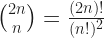
If ‘n’ is zero, this number is or 1. If ‘n’ is 1, this number is or 2. If ‘n’ is 2, this number is 6. If ‘n’ is 3, this number is (sparing the formula) 20. The numbers keep growing. 70, 252, 924, 3432, 12870, and so on.

So. 1 and 2 and 6 are squarefree numbers. Not much arguing that. But 20? That’s 2 squared times 5. 70? 2 times 5 times 7. 252? 2 squared times 3 squared times 7. 924? That’s 2 squared times 3 times 7 times 11. 3432? 2 cubed times 3 times 11 times 13; there’s a 2 squared in there. 12870? 2 times 3 squared times it doesn’t matter anymore. It’s not a squarefree number.

There’s a bunch of not-squarefree numbers in there. The question: do we ever stop seeing squarefree numbers here?

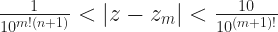
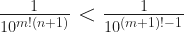
So here’s Sárközy’s Theorem. It says that this central binomial coefficient is never squarefree as long as ‘n’ is big enough. András Sárközy showed in 1985 that this was true. How big is big enough? … We have a bound, at least, for this theorem. If ‘n’ is larger than the number then the corresponding coefficient can’t be squarefree. It might not surprise you that the formulas involved here feature the Riemann Zeta function. That always seems to turn up for questions about large prime numbers.

That’s a common state of affairs for number theory problems. Very often we can show that something is true for big enough numbers. I’m not sure there’s a clear reason why. When numbers get large enough it can be more convenient to deal with their logarithms, I suppose. And those look more like the real numbers than the integers. And real numbers are typically easier to prove stuff about. Maybe that’s it. This is vague, yes. But to ask ‘why’ some things are easy and some are hard to prove is a hard question. What is a satisfying ’cause’ here?

It’s tempting to say that since we know this is true for all ‘n’ above a bound, we’re done. We can just test all the numbers below that bound, and the rest is done. You can do a satisfying proof this way: show that eventually the statement is true, and show all the special little cases before it is. This particular result is kind of useless, though. is a number that’s something like 241 digits long. For comparison, the total number of things in the universe is something like a number about 80 digits long. Certainly not more than 90. It’d take too long to test all those cases.

That’s all right. Since Sárközy’s proof in 1985 there’ve been other breakthroughs. In 1988 P Goetgheluck proved it was true for a big range of numbers: every ‘n’ that’s larger than 4 and less than . That’s a number something more than 12 million digits long. In 1991 I Vardi proved we had no squarefree central binomial coefficients for ‘n’ greater than 4 and less than , which is a number about 233 million digits long. And then in 1996 Andrew Granville and Olivier Ramare showed directly that this was so for all ‘n’ larger than 4.

So that 70 that turned up just a few lines in is the last squarefree one of these coefficients.

Is this surprising? Maybe, maybe not. I’ll bet most of you didn’t have an opinion on this topic twenty minutes ago. Let me share something that did surprise me, and continues to surprise me. In 1974 David Singmaster proved that any integer divides almost all the binomial coefficients out there. “Almost all” is here a term of art, but it means just about what you’d expect. Imagine the giant list of all the numbers that can be binomial coefficients. Then pick any positive integer you like. The number you picked will divide into so many of the giant list that the exceptions won’t be noticeable. So that square numbers like 4 and 9 and 16 and 25 should divide into most binomial coefficients? … That’s to be expected, suddenly. Into the central binomial coefficients? That’s not so obvious to me. But then so much of number theory is strange and surprising and not so obvious.

Words About A Wordless Induction Proof

This pair of tweets came across my feed. And who doesn’t like a good visual proof of a mathematical fact? I hope you enjoy.

So here’s the proposition.

Via @mathelegant pic.twitter.com/rX03qPo85n

— tchr (@egelizh) February 9, 2017

This is the sort of identity we normally try proving by induction. Induction is a great scheme for proving identities like this. It works by finding some index on the formula. Then show that if the formula is true for one value of the index, then it’s true for the next-higher value of the index. Finally, find some value of the index for which it’s easy to check that the formula’s true. And that proves it’s true for all the values of that index above that base.

In this case the index is ‘n’. It’s really easy to prove the base case, since 1³ is equal to 1² what with ‘1’ being the number everybody likes to raise to powers. Going from proving that if it’s true in one case — — then it’s true for the next — — is work. But you can get it done.

And then there’s this, done visually:

pic.twitter.com/bypK5PtTKQ

— tchr (@egelizh) March 5, 2017

It took me a bit to read fully until I was confident in what it was showing. But it is all there.

As often happens with these wordless proofs you can ask whether it is properly speaking a proof. A proof is an argument and to be complete it has to contain every step needed to deduce the conclusion from the premises, following one of the rules of inference each step. Thing is basically no proof is complete that way, because it takes forever. We elide stuff that seems obvious, confident that if we had to we could fill in the intermediate steps. A wordless proof like trusts that if we try to describe what is in the picture then we are constructing the argument.

That’s surely enough of my words.

Theorem Thursday: Liouville’s Approximation Theorem And How To Make Your Own Transcendental Number

As I get into the second month of Theorem Thursdays I have, I think, the whole roster of weeks sketched out. Today, I want to dive into some real analysis, and the study of numbers. It’s the sort of thing you normally get only if you’re willing to be a mathematics major. I’ll try to be readable by people who aren’t. If you carry through to the end and follow directions you’ll have your very own mathematical construct, too, so enjoy.

Liouville’s Approximation Theorem

It all comes back to polynomials. Of course it does. Polynomials aren’t literally everything in mathematics. They just come close. Among the things we can do with polynomials is divide up the real numbers into different sets. The tool we use is polynomials with integer coefficients. Integers are the positive and the negative whole numbers, stuff like ‘4’ and ‘5’ and ‘-12’ and ‘0’.

A polynomial is the sum of a bunch of products of coefficients multiplied by a variable raised to a power. We can use anything for the variable’s name. So we use ‘x’. Sometimes ‘t’. If we want complex-valued polynomials we use ‘z’. Some people trying to make a point will use ‘y’ or ‘s’ but they’re just showing off. Coefficients are just numbers. If we know the numbers, great. If we don’t know the numbers, or we want to write something that doesn’t commit us to any particular numbers, we use letters from the start of the alphabet. So we use ‘a’, maybe ‘b’ if we must. If we need a lot of numbers, we use subscripts: a₀, a₁, a₂, and so on, up to some a_n for some big whole number n. To talk about one of these without committing ourselves to a specific example we use a subscript of i or j or k: a_j, a_k. It’s possible that a_j and a_k equal each other, but they don’t have to, unless j and k are the same whole number. They might also be zero, but they don’t have to be. They can be any numbers. Or, for this essay, they can be any integers. So we’d write a generic polynomial f(x) as:

(Some people put the coefficients in the other order, that is, and so on. That’s not wrong. The name we give a number doesn’t matter. But it makes it harder to remember what coefficient matches up with, say, x¹⁴.)

A zero, or root, is a value for the variable (‘x’, or ‘t’, or what have you) which makes the polynomial equal to zero. It’s possible that ‘0’ is a zero, but don’t count on it. A polynomial of degree n — meaning the highest power to which x is raised is n — can have up to n different real-valued roots. All we’re going to care about is one.

Rational numbers are what we get by dividing one whole number by another. They’re numbers like 1/2 and 5/3 and 6. They’re numbers like -2.5 and 1.0625 and negative a billion. Almost none of the real numbers are rational numbers; they’re exceptional freaks. But they are all the numbers we actually compute with, once we start working out digits. Thus we remember that to live is to live paradoxically.

And every rational number is a root of a first-degree polynomial. That is, there’s some polynomial f(x) = a_0 + a_1 x that’s made zero for your polynomial. It’s easy to tell you what it is, too. Pick your rational number. You can write that as the integer p divided by the integer q. Now look at the polynomial f(x) = p – q x. Astounded yet?

That trick will work for any rational number. It won’t work for any irrational number. There’s no first-degree polynomial with integer coefficients that has the square root of two as a root. There are polynomials that do, though. There’s f(x) = 2 – x². You can find the square root of two as the zero of a second-degree polynomial. You can’t find it as the zero of any lower-degree polynomials. So we say that this is an algebraic number of the second degree.

This goes on higher. Look at the cube root of 2. That’s another irrational number, so no first-degree polynomials have it as a root. And there’s no second-degree polynomials that have it as a root, not if we stick to integer coefficients. Ah, but f(x) = 2 – x³? That’s got it. So the cube root of two is an algebraic number of degree three.

We can go on like this, although I admit examples for higher-order algebraic numbers start getting hard to justify. Most of the numbers people have heard of are either rational or are order-two algebraic numbers. I can tell you truly that the eighth root of two is an eighth-degree algebraic number. But I bet you don’t feel enlightened. At best you feel like I’m setting up for something. The number r(5), the smallest radius a disc can have so that five of them will completely cover a disc of radius 1, is eighth-degree and that’s interesting. But you never imagined the number before and don’t have any idea how big that is, other than “I guess that has to be smaller than 1”. (It’s just a touch less than 0.61.) I sound like I’m wasting your time, although you might start doing little puzzles trying to make smaller coins cover larger ones. Do have fun.

Liouville’s Approximation Theorem is about approximating algebraic numbers with rational ones. Almost everything we ever do is with rational numbers. That’s all right because we can make the difference between the number we want, even if it’s r(5), and the numbers we can compute with, rational numbers, as tiny as we need. We trust that the errors we make from this approximation will stay small. And then we discover chaos science. Nothing is perfect.

For example, suppose we need to estimate π. Everyone knows we can approximate this with the rational number 22/7. That’s about 3.142857, which is all right but nothing great. Some people know we can approximate it as 333/106. (I didn’t until I started writing this paragraph and did some research.) That’s about 3.141509, which is better. Then there’s 355/113, which is not as famous as 22/7 but is a celebrity compared to 333/106. That’s about 3.141529. Then we get into some numbers only mathematics hipsters know: 103993/33102 and 104348/33215 and so on. Fine.

The Liouville Approximation Theorem is about sequences that converge on an irrational number. So we have our first approximation x₁, that’s the integer p₁ divided by the integer q₁. So, 22 and 7. Then there’s the next approximation x₂, that’s the integer p₂ divided by the integer q₂. So, 333 and 106. Then there’s the next approximation yet, x₃, that’s the integer p₃ divided by the integer q₃. As we look at more and more approximations, x_j‘s, we get closer and closer to the actual irrational number we want, in this case π. Also, the denominators, the q_j‘s, keep getting bigger.

The theorem speaks of having an algebraic number, call it x, of some degree n greater than 1. Then we have this limit on how good an approximation can be. The difference between the number x that we want, and our best approximation p / q, has to be larger than the number (1/q)^{n + 1}. The approximation might be higher than x. It might be lower than x. But it will be off by at least the n-plus-first power of 1/q.

Polynomials let us separate the real numbers into infinitely many tiers of numbers. They also let us say how well the most accessible tier of numbers, rational numbers, can approximate these more exotic things.

One of the things we learn by looking at numbers through this polynomial screen is that there are transcendental numbers. These are numbers that can’t be the root of any polynomial with integer coefficients. π is one of them. e is another. Nearly all numbers are transcendental. But the proof that any particular number is one is hard. Joseph Liouville showed that transcendental numbers must exist by using continued fractions. But this approximation theorem tells us how to make our own transcendental numbers. This won’t be any number you or anyone else has ever heard of, unless you pick a special case. But it will be yours.

You will need:

1. a₁, an integer from 1 to 9, such as ‘1’, ‘9’, or ‘5’.
2. a₂, another integer from 1 to 9. It may be the same as a₁ if you like, but it doesn’t have to be.
3. a₃, yet another integer from 1 to 9. It may be the same as a₁ or a₂ or, if it so happens, both.
4. a₄, one more integer from 1 to 9 and you know what? Let’s summarize things a bit.
5. A whopping great big gob of integers a_j, every one of them from 1 to 9, for every possible integer ‘j’ so technically this is infinitely many of them.
6. Comfort with the notation n!, which is the factorial of n. For whole numbers that’s the product of every whole number from 1 to n, so, 2! is 1 times 2, or 2. 3! is 1 times 2 times 3, or 6. 4! is 1 times 2 times 3 times 4, or 24. And so on.
7. Not to be thrown by me writing -n!. By that I mean work out n! and then multiply that by -1. So -2! is -2. -3! is -6. -4! is -24. And so on.

Now, assemble them into your very own transcendental number z, by this formula:

If you’ve done it right, this will look something like:

Ah, but, how do you know this is transcendental? We can prove it is. The proof is by contradiction, which is how a lot of great proofs are done. We show nonsense follows if the thing isn’t true, so the thing must be true. (There are mathematicians that don’t care for proof-by-contradiction. They insist on proof by charging straight ahead and showing a thing is true directly. That’s a matter of taste. I think every mathematician feels that way sometimes, to some extent or on some issues. The proof-by-contradiction is easier, at least in this case.)

Suppose that your z here is not transcendental. Then it’s got to be an algebraic number of degree n, for some finite number n. That’s what it means not to be transcendental. I don’t know what n is; I don’t care. There is some n and that’s enough.

Now, let’s let z_m be a rational number approximating z. We find this approximation by taking the first m! digits after the decimal point. So, z₁ would be just the number 0.a₁. z₂ is the number 0.a₁a₂. z₃ is the number 0.a₁a₂000a₃. I don’t know what m you like, but that’s all right. We’ll pick a nice big m.

So what’s the difference between z and z_m? Well, it can’t be larger than 10 times 10^{-(m + 1)!}. This is for the same reason that π minus 3.14 can’t be any bigger than 0.01.

Now suppose we have the best possible rational approximation, p/q, of your number z. Its first m! digits are going to be p / 10^m!. This will be z_m And by the Liouville Approximation Theorem, then, the difference between z and z_m has to be at least as big as (1/10^m!)^{(n + 1)}.

So we know the difference between z and z_m has to be larger than one number. And it has to be smaller than another. Let me write those out.

We don’t need the z – z_m anymore. That thing on the rightmost side we can write what I’ll swear is a little easier to use. What we have left is:

And this will be true whenever the number m! (n + 1) is greater than (m + 1)! – 1 for big enough numbers m.

But there’s the thing. This isn’t true whenever m is greater than n. So the difference between your alleged transcendental number and its best-possible rational approximation has to be simultaneously bigger than a number and smaller than that same number without being equal to it. Supposing your number is anything but transcendental produces nonsense. Therefore, congratulations! You have a transcendental number.

If you chose all 1’s for your a_j‘s, then you have what is sometimes called the Liouville Constant. If you didn’t, you may have a transcendental number nobody’s ever noticed before. You can name it after someone if you like. That’s as meaningful as naming a star for someone and cheaper. But you can style it as weaving someone’s name into the universal truth of mathematics. Enjoy!

I’m glad to finally give you a mathematics essay that lets you make something you can keep.

Theorem Thursday: A First Fixed Point Theorem

I’m going to let the Mean Value Theorem slide a while. I feel more like a Fixed Point Theorem today. As with the Mean Value Theorem there’s several of these. Here I’ll start with an easy one.

The Fixed Point Theorem.

Back when the world and I were young I would play with electronic calculators. They encouraged play. They made it so easy to enter a number and hit an operation, and then hit that operation again, and again and again. Patterns appeared. Start with, say, ‘2’ and hit the ‘squared’ button, the smaller ‘2’ raised up from the key’s baseline. You got 4. And again: 16. And again: 256. And again and again and you got ever-huger numbers. This happened whenever you started from a number bigger than 1. Start from something smaller than 1, however tiny, and it dwindled down to zero, whatever you tried. Start at ‘1’ and it just stays there. The results were similar if you started with negative numbers. The first squaring put you in positive numbers and everything carried on as before.

This sort of thing happened a lot. Keep hitting the mysterious ‘exp’ and the numbers would keep growing forever. Keep hitting ‘sqrt’; if you started above 1, the numbers dwindled to 1. Start below and the numbers rise to 1. Or you started at zero, but who’s boring enough to do that? ‘log’ would start with positive numbers and keep dropping until it turned into a negative number. The next step was the calculator’s protest we were unleashing madness on the world.

But you didn’t always get zero, one, infinity, or madness, from repeatedly hitting the calculator button. Sometimes, some functions, you’d get an interesting number. If you picked any old number and hit cosine over and over the digits would eventually settle down to around 0.739085. Or -0.739085. Cosine’s great. Tangent … tangent is weird. Tangent does all sorts of bizarre stuff. But at least cosine is there, giving us this interesting number.

(Something you might wonder: this is the cosine of an angle measured in radians, which is how mathematicians naturally think of angles. Normal people measure angles in degrees, and that will have a different fixed point. We write both the cosine-in-radians and the cosine-in-degrees using the shorthand ‘cos’. We get away with this because people who are confused by this are too embarrassed to call us out on it. If we’re thoughtful we write, say, ‘cos x’ for radians and ‘cos x°’ for degrees. This makes the difference obvious. It doesn’t really, but at least we gave some hint to the reader.)

This all is an example of a fixed point theorem. Fixed point theorems turn up in a lot of fields. They were most impressed upon me in dynamical systems, studying how a complex system changes in time. A fixed point, for these problems, is an equilibrium. It’s where things aren’t changed by a process. You can see where that’s interesting.

In this series I haven’t stated theorems exactly much, and I haven’t given them real proofs. But this is an easy one to state and to prove. Start off with a function, which I’ll name ‘f’, because yes that is exactly how much effort goes in to naming functions. It has as a domain the interval [a, b] for some real numbers ‘a’ and ‘b’. And it has as rang the same interval, [a, b]. It might use the whole range; it might use only a subset of it. And we have to require that f is continuous.

Then there has to be at least one fixed point. There must be at last one number ‘c’, somewhere in the interval [a, b], for which f(c) equals c. There may be more than one; we don’t say anything about how many there are. And it can happen that c is equal to a. Or that c equals b. We don’t know that it is or that it isn’t. We just know there’s at least one ‘c’ that makes f(c) equal c.

You get that in my various examples. If the function f has the rule that any given x is matched to x², then we do get two fixed points: f(0) = 0² = 0, and, f(1) = 1² = 1. Or if f has the rule that any given x is matched to the square root of x, then again we have: and . Same old boring fixed points. The cosine is a little more interesting. For that we have .

How to prove it? The easiest way I know is to summon the Intermediate Value Theorem. Since I wrote a couple hundred words about that a few weeks ago I can assume you to understand it perfectly and have no question about how it makes this problem easy. I don’t even need to go on, do I?

… Yeah, fair enough. Well, here’s how to do it. We’ll take the original function f and create, based on it, a new function. We’ll dig deep in the alphabet and name that ‘g’. It has the same domain as f, [a, b]. Its range is … oh, well, something in the real numbers. Don’t care. The wonder comes from the rule we use.

The rule for ‘g’ is this: match the given number ‘x’ with the number ‘f(x) – x’. That is, g(a) equals whatever f(a) would be, minus a. g(b) equals whatever f(b) would be, minus b. We’re allowed to define a function in terms of some other function, as long as the symbols are meaningful. But we aren’t doing anything wrong like dividing by zero or taking the logarithm of a negative number or asking for f where it isn’t defined.

You might protest that we don’t know what the rule for f is. We’re told there is one, and that it’s a continuous function, but nothing more. So how can I say I’ve defined g in terms of a function I don’t know?

In the first place, I already know everything about f that I need to. I know it’s a continuous function defined on the interval [a, b]. I won’t use any more than that about it. And that’s great. A theorem that doesn’t require knowing much about a function is one that applies to more functions. It’s like the difference between being able to say something true of all living things in North America, and being able to say something true of all persons born in Redbank, New Jersey, on the 18th of February, 1944, who are presently between 68 and 70 inches tall and working on their rock operas. Both things may be true, but one of those things you probably use more.

In the second place, suppose I gave you a specific rule for f. Let me say, oh, f matches x with the arccosecant of x. Are you feeling any more enlightened now? Didn’t think so.

Back to g. Here’s some things we can say for sure about it. g is a function defined on the interval [a, b]. That’s how we set it up. Next point: g is a continuous function on the interval [a, b]. Remember, g is just the function f, which was continuous, minus x, which is also continuous. The difference of two continuous functions is still going to be continuous. (This is obvious, although it may take some considered thinking to realize why it is obvious.)

Now some interesting stuff. What is g(a)? Well, it’s whatever number f(a) is minus a. I can’t tell you what number that is. But I can tell you this: it’s not negative. Remember that f(a) has to be some number in the interval [a, b]. That is, it’s got to be no smaller than a. So the smallest f(a) can be is equal to a, in which case f(a) minus a is zero. And f(a) might be larger than a, in which case f(a) minus a is positive. So g(a) is either zero or a positive number.

(If you’ve just realized where I’m going and gasped in delight, well done. If you haven’t, don’t worry. You will. You’re just out of practice.)

What about g(b)? Since I don’t know what f(b) is, I can’t tell you what specific number it is. But I can tell you it’s not a positive number. The reasoning is just like above: f(b) is some number on the interval [a, b]. So the biggest number f(b) can equal is b. And in that case f(b) minus b is zero. If f(b) is any smaller than b, then f(b) minus b is negative. So g(b) is either zero or a negative number.

(Smiling at this? Good job. If you aren’t, again, not to worry. This sort of argument is not the kind of thing you do in Boring Algebra. It takes time and practice to think this way.)

And now the Intermediate Value Theorem works. g(a) is a positive number. g(b) is a negative number. g is continuous from a to b. Therefore, there must be some number ‘c’, between a and b, for which g(c) equals zero. And remember what g(c) means: f(c) – c equals 0. Therefore f(c) has to equal c. There has to be a fixed point.

And some tidying up. Like I said, g(a) might be positive. It might also be zero. But if g(a) is zero, then f(a) – a = 0. So a would be a fixed point. And similarly if g(b) is zero, then f(b) – b = 0. So then b would be a fixed point. The important thing is there must be at least some fixed point.

Now that calculator play starts taking on purposeful shape. Squaring a number could find a fixed point only if you started with a number from -1 to 1. The square of a number outside this range, such as ‘2’, would be bigger than you started with, and the Fixed Point Theorem doesn’t apply. Similarly with exponentials. But square roots? The square root of any number from 0 to a positive number ‘b’ is a number between 0 and ‘b’, at least as long as b was bigger than 1. So there was a fixed point, at 1. The cosine of a real number is some number between -1 and 1, and the cosines of all the numbers between -1 and 1 are themselves between -1 and 1. The Fixed Point Theorem applies. Tangent isn’t a continuous function. And the calculator play never settles on anything.

As with the Intermediate Value Theorem, this is an existence proof. It guarantees there is a fixed point. It doesn’t tell us how to find one. Calculator play does, though. Start from any old number that looks promising and work out f for that number. Then take that and put it back into f. And again. And again. This is known as “fixed point iteration”. It won’t give you the exact answer.

Not usually, anyway. In some freak cases it will. But what it will give, provided some extra conditions are satisfied, is a sequence of values that get closer and closer to the fixed point. When you’re close enough, then you stop calculating. How do you know you’re close enough? If you know something about the original f you can work out some logically rigorous estimates. Or you just keep calculating until all the decimal points you want stop changing between iterations. That’s not logically sound, but it’s easy to program.

That won’t always work. It’ll only work if the function f is differentiable on the interval (a, b). That is, it can’t have corners. And there have to be limits on how fast the function changes on the interval (a, b). If the function changes too fast, iteration can’t be guaranteed to work. But often if we’re interested in a function at all then these conditions will be true, or we can think of a related function that for which they are true.

And even if it works it won’t always work well. It can take an enormous pile of calculations to get near the fixed point. But this is why we have computers, and why we can leave them to work overnight.

And yet such a simple idea works. It appears in ancient times, in a formula for finding the square root of an arbitrary positive number ‘N’. (Find the fixed point for ). It creeps into problems that don’t look like fixed points. Calculus students learn of something called the Newton-Raphson Iteration. It finds roots, points where a function f(x) equals zero. Mathematics majors learn of numerical methods to solve ordinary differential equations. The most stable of these are again fixed-point iteration schemes, albeit in disguise.

They all share this almost playful backbone.

A Picture Showing Why The Square Root of 2 Is Irrational

Seyma Erbas had a post recently that I quite liked. It’s a nearly visual proof of the irrationality of the square root of two. Proving that the square root of two is irrational isn’t by itself a great trick: either that or the proof there are infinitely many prime numbers is probably the simplest interesting proof-by-contradiction someone could do. The Pythagoreans certainly knew of it, and being the Pythagoreans, inspired confusing legends about just what they did about this irrationality.

Anyway, in the reblogged post here, a proof (by contradiction) that the square root of two can’t be rational is done nearly entirely in pictures. The paper which Seyma Erbas cites, Steven J Miller and David Montague’s “Irrationality From The Book”, also includes similar visual proofs of the irrationality of the square roots of three, five, and six, and if the pictures don’t inspire you to higher mathematics they might at least give you ideas for retiling the kitchen. Miller and Montague talk about the generalization problem — making similar diagrams for larger and larger numbers, such as ten — and where their generalization stops working.

Seyma Erbas

Yesterday I came a across a new (new to me, that is) proof of the irrationality of . I found it in the paper “Irrationality From The Book,” by Steven J. Miller, David Montague, which was recently posted to arXiv.org.

Apparently the proof was discovered by Stanley Tennenbaum in the 1950′s but was made widely known by John Conway around 1990. The proof appeared in Conway’s chapter “The Power of Mathematics” of the book Power, which was edited by Alan F. Blackwell, David MacKay (2005).

View original post 213 more words

Emile Lemoine

Through the MacTutor archive I learn that today’s the birthday of Émile Michel Hyacinthe Lemoine (1840 – 1912), a mathematician I admit I don’t remember hearing of before. His particular mathematical interests were primarily in geometry (though MacTutor notes professionally he became a civil engineer responsible for Paris’s gas supply).

What interests me is that Lemoine looked into the problem of how complicated a proof is, and in just the sort of thing designed to endear him to my heart, he tried to give a concrete measurement of, at least, how involved a geometric construction was. He identified the classic steps in compass-and-straightedge constructions and classified proofs by how many steps these took. MacTutor cites him as showing that the usual solution to the Apollonius problem — construct a circle tangent to three given circles — required over four hundred operations, but that he was able to squeeze that down to 199.

However, well, nobody seems to have been very interested in this classification. That’s probably because the length doesn’t really measure how complicated a proof (or a construction) is: proofs can have a narrative flow, and a proof that involves many steps each of which seems to flow obviously (or which look like the steps in another, already-familiar proof) is going to be easier to read and to understand than one that involves fewer but more obscure steps. This is the sort of thing that challenges attempts to measure how difficult a proof is, even though it’d be interesting to know.

Here’s one of the things that would be served by being able to measure just how long a proof is: a lot of numerical mathematics depends on having sequences of randomly generated numbers, but, showing that you actually have a random sequence of numbers is a deeply hard problem. If you can specify how you get a particular digit … well, they’re not random, then, are they? Unless it’s “use this digit from this randomly generated sequence”. If you could show there’s no way to produce a particular sequence of numbers in any way more efficiently than just reading them off this list of numbers you’d at least have a fair chance at saying this is a truly unpredictable sequence. But, showing that you have found the most efficient algorithm for producing something is … well, it’s difficult to even start measuring that sort of thing, and while Lemoine didn’t produce a very good measure of algorithmic complexity, he did have an idea, and it’s difficult to see how one could get a good measure if one didn’t start with trying not-very-good ones.

Eliminating Your Footprints

When last we discussed divisibility rules, particularly, rules for just adding up the digits in a number to tell what it might divide by, we had worked out rules for testing divisibility by eight. In that, we take the sum of four times the hundreds digit, plus two times the tens digit, plus the units digit, and if that sum is divisible by eight, then so was the original number. This hasn’t got the slick, smooth memorability of the rules for three and nine — just add all the numbers up — or the simplicity of checking for divisibility by ten, five, or two — just look at the last digit — but it’s not a complicated rule either.

Still, we came at it through an experimental method, fiddling around with possible rules until we found one which seemed to work. It seemed to work, and since we found out there are only a thousand possible cases to consider we can check that it works in every one of those cases. That’s tiresome to do, but functions, and it’s a legitimate way of forming mathematical rules. Quite a number of proofs amount to dividing a problem into several different cases and show that whatever we mean to prove is so in each ase.

Let’s see what we can do to tidy up the proof, though, and see if we can make it work without having to test out so many cases. We can, or I’d have been foolish to start this essay rather than another; along the way, though, we can remove the traces that show the experimenting that lead to the technique. We can put forth the cleaned-up reasoning and look all the more clever because it isn’t so obvious how we got there. This is another common property of proofs; the most attractive or elegant method of presenting them can leave the reader wondering how it was ever imagined.