What we mean by that is the area between some left boundary, , and some right boundary, , that’s above the x-axis, and below that curve. And there’s just no finding a, you know, answer. Something that looks like (to make up an answer) the area is or something normal like that. The one interesting exception is that you can find the area if the left bound is and the right bound . That’s done by some clever reasoning and changes of variables which is why we see that and only that in freshman calculus. (Oh, and as a side effect we can get the integral between 0 and infinity, because that has to be half of that.)
Anyway, Quintanilla includes a nice bit along the way, that I don’t remember from my freshman calculus, pointing out why we can’t come up with a nice simple formula like that. It’s a loose argument, showing what would happen if we suppose there is a way to integrate this using normal functions and showing we get a contradiction. A proper proof is much harder and fussier, but this is likely enough to convince someone who understands a bit of calculus and a bit of Taylor series.
I got a good nomination for a Q topic, thanks again to goldenoj. It was for Qualitative/Quantitative. Either would be a good topic, but they make a natural pairing. They describe the things mathematicians look for when modeling things. But ultimately I couldn’t find an angle that I liked. So rather than carry on with an essay that wasn’t working I went for a topic of my own. Might come back around to it, though, especially if nothing good presents itself for the letter X, which will probably need to be a wild card topic anyway.
We like comparing sizes. I talked about that some with norms. We do the same with shapes, though. We’d like to know which one is bigger than another, and by how much. We rely on squares to do this for us. It could be any shape, but we in the western tradition chose squares. I don’t know why.
My guess, unburdened by knowledge, is the ancient Greek tradition of looking at the shapes one can make with straightedge and compass. The easiest shape these tools make is, of course, circles. But it’s hard to find a circle with the same area as, say, any old triangle. Squares are probably a next-best thing. I don’t know why not equilateral triangles or hexagons. Again I would guess that the ancient Greeks had more rectangular or square rooms than the did triangles or hexagons, and went with what they knew.
So that’s what lurks behind that word “quadrature”. It may be hard for us to judge whether this pentagon is bigger than that octagon. But if we find squares that are the same size as the pentagon and the octagon, great. We can spot which of the squares is bigger, and by how much.
Straightedge-and-compass lets you find the quadrature for many shapes. Like, take a rectangle. Let me call that ABCD. Let’s say that AB is one of the long sides and BC one of the short sides. OK. Extend AB, outwards, to another point that I’ll call E. Pick E so that the length of BE is the same as the length of BC.
Next, bisect the line segment AE. Call that point F. F is going to be the center of a new semicircle, one with radius FE. Draw that in, on the side of AE that’s opposite the point C. Because we are almost there.
Extend the line segment CB upwards, until it touches this semicircle. Call the point where it touches G. The line segment BG is the side of a square with the same area as the original rectangle ABCD. If you know enough straightedge-and-compass geometry to do that bisection, you know enough to turn BG into a square. If you’re not sure why that’s the correct length, you can get there quickly. Use a little algebra and the Pythagorean theorem.
Neat, yeah, I agree. Also neat is that you can use the same trick to find the area of a parallelogram. A parallelogram has the same area as a square with the same bases and height between them, you remember. So take your parallelogram, draw in some perpendiculars to share that off into a rectangle, and find the quadrature of that rectangle. you’ve got the quadrature of your parallelogram.
Having the quadrature of a parallelogram lets you find the quadrature of any triangle. Pick one of the sides of the triangle as the base. You have a third point not on that base. Draw in the parallel to that base that goes through that third point. Then choose one of the other two sides. Draw the parallel to that side which goes through the other point. Look at that: you’ve got a parallelogram with twice the area of your original triangle. Bisect either the base or the height of this parallelogram, as you like. Then follow the rules for the quadrature of a parallelogram, and you have the quadrature of your triangle. Yes, you’re doing a lot of steps in-between the triangle you started with and the square you ended with. Those steps don’t count, not by this measure. Getting the results right matters.
And here’s some more beauty. You can find the quadrature for any polygon. Remember how you can divide any polygon into triangles? Go ahead and do that. Find the quadrature for every one of those triangles then. And you can create a square that has an area as large as all those squares put together. I’ll refrain from saying quite how, because realizing how is such a delight, one of those moments that at least made me laugh at how of course that’s how. It’s through one of those things that even people who don’t know mathematics know about.
With that background you understand why people thought the quadrature of the circle ought to be possible. Moreso when you know that the lune, a particular crescent-moon-like shape, can be squared. It looks so close to a half-circle that it’s obvious the rest should be possible. It’s not, and it took two thousand years and a completely different idea of geometry to prove it. But it sure looks like it should be possible.
Along the way to modernity quadrature picked up a new role. This is as part of calculus. One of the legs of calculus is integration. There is an interpretation of what the (definite) integral of a function means so common that we sometimes forget it doesn’t have to be that. This is to say that the integral of a function is the area “underneath” the curve. That is, it’s the area bounded by the limits of integration, by the horizontal axis, and by the curve represented by the function. If the function is sometimes less than zero, within the limits of integration, we’ll say that the integral represents the “net area”. Then we allow that the net area might be less than zero. Then we ignore the scolding looks of the ancient Greek mathematicians.
No matter. We love being able to find “the” integral of a function. This is a new function, and evaluating it tells us what this net area bounded by the limits of integration is. Finding this is “integration by quadrature”. At least in books published back when they wrote words like “to-day” or “coördinate”. My experience is that the term’s passed out of the vernacular, at least in North American Mathematician’s English.
Anyway the real flaw is that there are, like, six functions we can find the integral for. For the rest, we have to make do with approximations. This gives us “numerical quadrature”, a phrase which still has some currency.
And with my prologue about compass-and-straightedge quadrature you can see why it’s called that. Numerical integration schemes often rely on finding a polynomial with a part that looks like a graph of the function you’re interested in. The other edges look like the limits of the integration. Then the area of that polygon should be close to the area “underneath” this function. So it should be close to the integral of the function you want. And we’re old hands at how the quadrature of polygons, since we talked that out like five hundred words ago.
Now, no person ever has or ever will do numerical quadrature by compass-and-straightedge on some function. So why call it “numerical quadrature” instead of just “numerical integration”? Style, for one. “Quadrature” as a word has a nice tone, clearly jargon but not threateningly alien. Also “numerical integration” often connotes the solving differential equations numerically. So it can clarify whether you’re evaluating integrals or solving differential equations. If you think that’s a distinction worth making. Evaluating integrals and solving differential equations are similar together anyway.
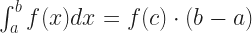
And there is another adjective that often attaches to quadrature. This is Gaussian Quadrature. Gaussian Quadrature is, in principle, a fantastic way to do numerical integration perfectly. For some problems. For some cases. The insight which justifies it to me is one of those boring little theorems you run across in the chapter introducing How To Integrate. It runs something like this. Suppose ‘f’ is a continuous function, with domain the real numbers and range the real numbers. Suppose a and b are the limits of integration. Then there’s at least one point c, between a and b, for which:
So if you could pick the right c, any integration would be so easy. Evaluate the function for one point and multiply it by whatever b minus a is. The catch is, you don’t know what c is.
Except there’s some cases where you kinda do. Like, if f is a line, rising or falling with a constant slope from a to b? Then have c be the midpoint of a and b.
That won’t always work. Like, if f is a parabola on the region from a to b, then c is not going to be the midpoint. If f is a cubic, then the midpoint is probably not c. And so on. And if you don’t know what kind of function f is? There’s no guessing where c will be.
But. If you decide you’re only trying to certain kinds of functions? Then you can do all right. If you decide you only want to integrate polynomials, for example, then … well, you’re not going to find a single point c for this. But what you can find is a set of points between a and b. Evaluate the function for those points. And then find a weighted average by rules I’m not getting into here. And that weighted average will be exactly that integral.
Of course there’s limits. The Gaussian Quadrature of a function is only possible if you can evaluate the function at arbitrary points. If you’re trying to integrate, like, a set of sample data it’s inapplicable. The points you pick, and the weighting to use, depend on what kind of function you want to integrate. The results will be worse the less your function is like what you supposed. It’s tedious to find what these points are for a particular assumption of function. But you only have to do that once, or look it up, if you know (say) you’re going to use polynomials of degree up to six or something like that.
And there are variations on this. They have names like the Chevyshev-Gauss Quadrature, or the Hermite-Gauss Quadrature, or the Jacobi-Gauss Quadrature. There are even some that don’t have Gauss’s name in them at all.
Despite that, you can get through a lot of mathematics not talking about quadrature. The idea implicit in the name, that we’re looking to compare areas of different things by looking at squares, is obsolete. It made sense when we worked with numbers that depended on units. One would write about a shape’s area being four times another shape’s, or the length of its side some multiple of a reference length.
We’ve grown comfortable thinking of raw numbers. It makes implicit the step where we divide the polygon’s area by the area of some standard reference unit square. This has advantages. We don’t need different vocabulary to think about integrating functions of one or two or ten independent variables. We don’t need wordy descriptions like “the area of this square is to the area of that as the second power of this square’s side is to the second power of that square’s side”. But it does mean we don’t see squares as intermediaries to understanding different shapes anymore.
If you take any positive integer n and sum the squares of its digits, repeating this operation, eventually you’ll either end at 1 or cycle between the eight values 4,16,37,58,89,145,42 and 20.
This one I saw through John Allen Paulos’s twitter feed. He points out that it’s like the Collatz conjecture but is, in fact, proven. If you try this yourself don’t make the mistake of giving up too soon. You might figure, like start with 12. Sum the squares of its digits and you get 5, which is neither 1 nor anything in that 4-16-37-58-89-145-42-20 cycle. Not so! Square 5 and you get 25. Square those digits and add them and you get 29. Square those digits and add them and you get 40. And what comes next?
This is about a proof of Fermat’s Theorem of Sums of Two Squares. According to it, a prime number — let’s reach deep into the alphabet and call it p — can be written as the sum of two squares if and only if p is one more than a whole multiple of four. It’s a proof by using fixed point methods. This is a fun kind of proof, at least to my sense of fun. It’s an approach that’s got a clear physical interpretation. Imagine picking up a (thin) patch of bread dough, stretching it out some and maybe rotating it, and then dropping it back on the board. There’s at least one bit of dough that’s landed in the same spot it was before. Once you see this you will never be able to just roll out dough the same way. So here the proof involves setting up an operation on integers which has a fixed point, and that the fixed point makes the property true.
John D Cook, who runs a half-dozen or so mathematics-fact-of-the-day Twitter feeds, looks into calculating the volume of an egg. It involves calculus, as finding the volume of many interesting shapes does. I am surprised to learn the volume can be written out as a formula that depends on the shape of the egg. I would have bet that it couldn’t be expressed in “closed form”. This is a slightly flexible term. It’s meant to mean the thing can be written using only normal, familiar functions. However, we pretend that the inverse hyperbolic tangent is a “normal, familiar” function.
For example, there’s the surface area of an egg. This can be worked out too, again using calculus. It can’t be written even with the inverse hyperbolic cotangent, so good luck. You have to get into numerical integration if you want an answer humans can understand.
Stand on the edge of a plot of land. Walk along its boundary. As you walk the edge pay attention. Note how far you walk before changing direction, even in the slightest. When you return to where you started consult your notes. Contained within them is the area you circumnavigated.
If that doesn’t startle you perhaps you haven’t thought about how odd that is. You don’t ever touch the interior of the region. You never do anything like see how many standard-size tiles would fit inside. You walk a path that is as close to one-dimensional as your feet allow. And encoded in there somewhere is an area. Stare at that incongruity and you realize why integrals baffle the student so. They have a deep strangeness embedded in them.
We who do mathematics have always liked integration. They grow, in the western tradition, out of geometry. Given a shape, what is a square that has the same area? There are shapes it’s easy to find the area for, given only straightedge and compass: a rectangle? Easy. A triangle? Just as straightforward. A polygon? If you know triangles then you know polygons. A lune, the crescent-moon shape formed by taking a circular cut out of a circle? We can do that. (If the cut is the right size.) A circle? … All right, we can’t do that, but we spent two thousand years trying before we found that out for sure. And we can do some excellent approximations.
That bit of finding-a-square-with-the-same-area was called “quadrature”. The name survives, mostly in the phrase “numerical quadrature”. We use that to mean that we computed an integral’s approximate value, instead of finding a formula that would get it exactly. The otherwise obvious choice of “numerical integration” we use already. It describes computing the solution of a differential equation. We’re not trying to be difficult about this. Solving a differential equation is a kind of integration, and we need to do that a lot. We could recast a solving-a-differential-equation problem as a find-the-area problem, and vice-versa. But that’s bother, if we don’t need to, and so we talk about numerical quadrature and numerical integration.
Integrals are built on two infinities. This is part of why it took so long to work out their logic. One is the infinity of number; we find an integral’s value, in principle, by adding together infinitely many things. The other is an infinity of smallness. The things we add together are infinitesimally small. That we need to take things, each smaller than any number yet somehow not zero, and in such quantity that they add up to something, seems paradoxical. Their geometric origins had to be merged into that of arithmetic, of algebra, and it is not easy. Bishop George Berkeley made a steady name for himself in calculus textbooks by pointing this out. We have worked out several logically consistent schemes for evaluating integrals. They work, mostly, by showing that we can make the error caused by approximating the integral smaller than any margin we like. This is a standard trick, or at least it is, now that we know it.
That “in principle” above is important. We don’t actually work out an integral by finding the sum of infinitely many, infinitely tiny, things. It’s too hard. I remember in grad school the analysis professor working out by the proper definitions the integral of 1. This is as easy an integral as you can do without just integrating zero. He escaped with his life, but it was a close scrape. He offered the integral of x as a way to test our endurance, without actually doing it. I’ve never made it through that.
But we do integrals anyway. We have tools on our side. We can show, for example, that if a function obeys some common rules then we can use simpler formulas. Ones that don’t demand so many symbols in such tight formation. Ones that we can use in high school. Also, ones we can adapt to numerical computing, so that we can let machines give us answers which are near enough right. We get to choose how near is “near enough”. But then the machines decide how long we’ll have to wait to get that answer.
The greatest tool we have on our side is the Fundamental Theorem of Calculus. Even the name promises it’s the greatest tool we might have. This rule tells us how to connect integrating a function to differentiating another function. If we can find a function whose derivative is the thing we want to integrate, then we have a formula for the integral. It’s that function we found. What a fantastic result.
The trouble is it’s so hard to find functions whose derivatives are the thing we wanted to integrate. There are a lot of functions we can find, mind you. If we want to integrate a polynomial it’s easy. Sine and cosine and even tangent? Yeah. Logarithms? A little tedious but all right. A constant number raised to the power x? Also tedious but doable. A constant number raised to the power x2? Hold on there, that’s madness. No, we can’t do that.
There is a weird grab-bag of functions we can find these integrals for. They’re mostly ones we can find some integration trick for. An integration trick is some way to turn the integral we’re interested in into a couple of integrals we can do and then mix back together. A lot of a Freshman Calculus course is a heap of tricks we’ve learned. They have names like “u-substitution” and “integration by parts” and “trigonometric substitution”. Some of them are really exotic, such as turning a single integral into a double integral because that leads us to something we can do. And there’s something called “differentiation under the integral sign” that I don’t know of anyone actually using. People know of it because Richard Feynman, in his fun memoir What Do You Care What Other People Think: 250 Pages Of How Awesome I Was In Every Situation Ever, mentions how awesome it made him in so many situations. Mathematics, physics, and engineering nerds are required to read this at an impressionable age, so we fall in love with a technique no textbook ever mentions. Sorry.
I’ve written about all this as if we were interested just in areas. We’re not. We like calculating lengths and volumes and, if we dare venture into more dimensions, hypervolumes and the like. That’s all right. If we understand how to calculate areas, we have the tools we need. We can adapt them to as many or as few dimensions as we need. By weighting integrals we can do calculations that tell us about centers of mass and moments of inertial, about the most and least probable values of something, about all quantum mechanics.
As often happens, this powerful tool starts with something anyone might ponder: what size square has the same area as this other shape? And then think seriously about it.
A friend took me up last night on my offer to help with any mathematics she was unsure about. I’m happy to do it, though of course it came as I was trying to shut things down for bed. But that part was inevitable and besides the exam was today. I thought it worth sharing here, though.
There’s going to be some calculus in this. There’s no avoiding that. If you don’t know calculus, relax about what the symbols exactly mean. It’s a good trick. Pretend anything you don’t know is just a symbol for “some mathematics thingy I can find out about later, if I need to, and I don’t necessarily have to”.
“Integration by parts” is one of the standard tricks mathematicians learn in calculus. It comes in handy if you want to integrate a function that itself looks like the product of two other functions. You find the integral of a function by breaking it up into two parts, one of which you differentiate and one of which you integrate. This gives you a product of functions and then a new integral to do. A product of functions is easy to deal with. The new integral … well, if you’re lucky, it’s an easier integral than you started with.
As you learn integration by parts you learn to look ways to break up functions so the new integral is easier. There’s no hard and fast rule for this. But bet on “the part that has a polynomial in it” as the part that’s better differentiated. “The part that has sines and cosines in it” is probably the part that’s better integrated. An exponential, like 2x, is as easily differentiated as integrated. The exponential of a function, like say 2x2, is better differentiated. These usually turn out impossible to integrate anyway. At least impossible without using crazy exotic functions.
So your classic integration-by-parts problem gives you an expression like this:
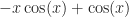
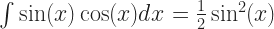
If you weren’t a mathematics major that might not look better to you, what with it still having integrals and sines and stuff in it. But ask your mathematics friend. She’ll tell you. The thing on the right-hand side is way better. That last term, the integral of the sine of x? She can do that in her sleep. It barely counts as work, at least by the time you’ve got in class to doing integration by parts. It’ll be .
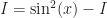
But sometimes, especially if the function being integrated — the “integrand”, by the way, and good luck playing that in Scrabble — is a bunch of trig functions and exponentials, you get some sad situation like so:
That is, the thing we wanted to integrate, on the left, turns up on the right too. The student sits down, feeling the futility of modern existence. We’re stuck with the original problem all over again and we’re short of tools to do something about it.
This is the point my friend was confused by, and is the bit of dark magic I want to talk about here. We’re not stumped! We can fall back on one of those mathematics tricks we are always allowed to do. And it’s a trick that’s so simple it seems like it can’t do anything.
It’s substitution. We are always allowed to substitute one thing for something else that’s equal to it. So in that above equation, what can we substitute, and for what? … Well, nothing in that particular bunch of symbols. We’re going to introduce a new one. It’s going to be the value of the integral we want to evaluate. Since it’s an integral, I’m going to call it ‘I’. You don’t have to call it that, but you’re going to anyway. It doesn’t need a more thoughtful name.
So I shall define:
The triple-equals-sign there is an extravagance, I admit. But it’s a common one. Mathematicians use it to say “this is defined to be equal to that”. Granted, that’s what the = sign means. But the triple sign connotes how we emphasize the definition part. That is, ‘I’ might have been anything at all, and we choose this of the universe of possibilities.
How does this help anything? Well, it turns the integration-by-parts problem into this equation:
And we want to know what ‘I’ equals. And now suddenly it’s easier to see that we don’t actually have to do any calculus from here on out. We can solve it the way we’d solve any problem in high school algebra, which is, move ‘I’ to the other side. Formally, we add the same thing to the left- and the right-hand sides. That’s ‘I’ …
… and then divide both sides by the same number, 2 …
And now remember that substitution is a free action. We can do it whenever we like, and we can undo it whenever we like. This is a good time to undo it. Putting the whole expression back in for ‘I’ we get …
… which is the integral, evaluated.
(Someone would like to point out there should be a ‘plus C’ in there. This someone is right, for reasons that would take me too far afield to describe right now. We can overlook it for now anyway. I just want that someone to know I know what you’re thinking and you’re not catching me on this one.)
Sometimes, the integration by parts will need two or even three rounds before you get back the original integrand. This is because the instructor has chosen a particularly nasty problem for homework or the exam. It is not hopeless! But you will see strange constructs like 4/5 I equalling something. Carry on.
What makes this a bit of dark magic? I think it’s because of habits. We write down something simple on the left-hand side of an equation. We get an expression for what the right-hand side should be, and it’s usually complicated. And then we try making the right-hand side simpler and simpler. The left-hand side started simple so we never even touch it again. Indeed, working out something like this it’s common to write the left-hand side once, at the top of the page, and then never again. We just write an equals sign, underneath the previous line’s equals sign, and stuff on the right. We forget the left-hand side is there, and that we can do stuff with it and to it.
I think also we get into a habit of thinking an integral and integrand and all that is some quasi-magic mathematical construct. But it isn’t. It’s just a function. It may even be just a number. We don’t know what it is, but it will follow all the same rules of numbers, or functions. Moving it around may be more writing but it’s not different work to moving ‘4’ or ‘x2‘ around. That’s the value of replacing the integral with a symbol like ‘I’. It’s not that there’s something we can do with ‘I’ that we can’t do with ‘‘, other than write it in under four pen strokes. It’s that in algebra we learned the habit of moving a letter around to where it’s convenient. Moving a whole integral expression around seems different.
But it isn’t. It’s the same work done, just on a different kind of mathematics. I suspect finding out that it could be a trick that simple throws people off.
It’s been a normal cluster of mathematically-themed jokes this past week. But one of them lets me show off my ability to do introductory calculus.
Norm Feuti’s Gil for the 15th of March is a resisting-the-word-problems joke. It’s also a rerun, sad to say. King Features syndicated Feuti’s strip for a couple of years, but couldn’t make a go of it. GoComics.com is reprinting what ran and that’s something, at least.
Justin Boyd’s Invisible Bread for the 16th plays on alarm clocks that make you solve problems. I’ve heard of these things, and I suppose they exist or something. The idea is that making you do a bit of arithmetic proves you’ve gotten up enough to not fall right back asleep. The clockmakers are underestimating my ability to get back to sleep. Anyway, I like the escalation of this.
The integral that has to be solved, , is a good problem for people taking their first calculus course. Let me spoil it as a homework problem by saying how I’d solve it. If you haven’t got the first idea what calculus is about and don’t wish to know, go ahead and skip to the bit about Rudy Park. Or just enjoy the parts of the sentences below that aren’t mathematics.
The first thing I notice is the integrand, the thing inside the integral. That’s , which is the same as . Distributive law, as if you didn’t know. That strikes me as worth doing because, if the integral converges, the integral of the sum of two things is the same as the sum of the integral of two things. I’m willing to suppose it converges until given evidence otherwise. So this integral is the same as .
I think that’s worth doing because that first integral is incredibly easy. It’ll be a number equal to whatever -e-x is, when x is infinitely large, minus what -e-x is when x is zero. When x is infinitely large, -e-x is zero. When x is 0, -e-x is -1. So 0 minus -1 is … 1.
is harder. But it suggests how to evaluate it. The integrand is the quantity 2x times the quantity e-x. 2x is easy to take the derivative of. e-x is easy to integrate. (It’s also easy to take the derivative of, but it’s easier to integrate.) This suggests trying out integration by parts.
When you integrate by parts, you notice the original integral is the product of a part that’s easy to differentiate and a part that’s easy to integrate. My Intro Calculus textbooks generically label the easy-to-differentiate part u, and the easy-to-integrate part dv. Then the derivatie of the easy-to-differentiate part is du, and the integral of the easy-to-integrate part is v. When you integrate by parts, the integral of u times dv turns out to be equal to u times v (no integral signs there) minus the integral of v du. This may sound like we’ve just turned one integral into another. So we have. But we’ve often made it into an easier integral to evaluate. This is why we ever try it.
So if u equals 2x, then its derivative du is equal to 2 dx. If dv is equal to e-xdx (we want to carry those little d’s along), then v is equal to -e-x. And this means we have this:
.
That middle part, , is not an integral. It’s been integrated. The notation there means to evaluate the thing when x is infinitely large, and evaluate the thing when x is zero. Then subtract the x-is-zero value from the x-is-infinitely-large value. The x-is-zero value of this expression turns out to be zero, as you realize when you start writing “2 times 0 times oh wait we’re done here”. The x-is-infinitely-large value of this expression takes longer to get done. If you want to do it right you have to invoke l’Hôpital’s Rule. But it’s also zero.
The right-hand part, , is equal to , and that’s equal to . Which will be 0 minus a -2. Or 2 altogether.
So the integral is 1 plus 2, or in total, 3. The strip got its integration right.
Darrin Bell and Theron Heir’s Rudy Park for the 16th speaks of some architect who said the job didn’t demand being good at mathematics. I hadn’t heard the original claim and didn’t feel my constitution up to finding it. It was hard enough reading the comments at GoComics.com.
Ruben Bolling’s Super-Fun-Pak Comix for the 17th has found a weakness in my policy of “we’ve maybe done enough Chaos Butterfly and Schrödinger’s Cat mantions”.
Mark Anderson’s Andertoons for the 18th mentions circle and radius and that’s all Mark Anderson needs to get my publicity.
David L Hoyt and Jeff Knurek’s Jumble for the 18th has an arithmetic theme. Note the quote marks in the final answer. They’re a warning that the punch line is a pun or wordplay.
I’ve been on a bit of a logarithms kick lately, and I should say I’m not the only one. HowardAt58 has had a good number of articles about it, too, and I wanted to point some out to you. In this particular reblogging he brings a bit of calculus to show why the logarithm of the product of two numbere has to be the sum of the logarithms of the two separate numbers, in a way that’s more rigorous (if you’re comfortable with freshman calculus) than just writing down a couple examples along the lines of how 102 times 103 is equal to 105. (I won’t argue that having a couple specific examples might be better at communicating the point, but there’s a difference between believing something is so and being able to prove that it’s true.)
The derivative of the log function can be investigated informally, as log(x) is seen as the inverse of the exponential function, written here as exp(x). The exponential function appears naturally from numbers raised to varying powers, but formal definitions of the exponential function are difficult to achieve. For example, what exactly is the meaning of exp(pi) or exp(root(2)).
So we look at the log function:-
I have a guest post that I mean to put up shortly which is a spinoff of the talk last month about calculating logarithms. There are several ways to define a logarithm but one of the most popular is to define it as an integral. That has the advantages of allowing the logarithm to be studied using a lot of powerful analytic tools already built up for calculus, and allow it to be calculated numerically because there are a lot of methods for calculating logarithms out there. I wanted to precede that post with a discussion of a couple of the ways to do these numerical integrations.
A great way to interpret integrating a function is to imagine drawing a plot of function; the integral is the net area between the x-axis and the plot of that function. That may be pretty hard to do, though, so we fall back on a standard mathematician’s trick that they never tell you about in grade school, probably for good reason: don’t bother doing the problem you actually have, and instead do a problem that looks kind of like it but that you are able to do.
Normally, for what’s called a definite integral, we’re interested in the area underneath a curve and across an “interval”, that is, between some minimum and some maximum value on the x-axis. Definite integrals are the kind we can approximate numerically. An indefinite integral gives a function that would tell us what the definite integral on any interval would be, but that takes symbolic mathematics to work out and that’s way beyond this article’s scope.
The red curve here represents some function. Any function will do, really. This is just one of them.
While we may have no idea what the area underneath a complicated squiggle on some interval is, we do know what the area inside a rectangle is. So if we pretend we’re interested in the area of the rectangle instead of the original area, good. Take my little drawing of a generic function here, the wavey red curve. The integral of it from wherever that left vertical green line is to the right is the area between the x-axis, the horizontal black line, and the red curve.
For the Rectangle Rule, find the area of a rectangle that approximates the function whose integral you’re actually interested in. Shown here are the left-endpoint (yellow line) and the right-endpoint (blue line) approximations, but any rule can be used to find the approximation.
If we use the “Rectangle Rule”, we draw a horizontal line based on the value of the function somewhere from the left line to the right. The yellow line up top is based on the value at the left endpoint. The blue line is based on the value the function has at the right endpoint. We can use any point, although the most popular ones are the left endpoint, the right endpoint, and the midpoint, because those are nice, easy picks to make. (And if we’re trying to integrate a function whose definition we don’t know, for example because it’s the data we got from an experiment, these will often be the only data points we have.) The area under the curve is going to be something like the area of the rectangle bounded by the green lines, the horizontal black line, and the blue horizontal line or the yellow horizontal line.
Drawn this way you might complain this approximation is rubbish: the area of the blue-topped rectangle is obviously way too low, and that of the yellow-topped rectangle is way too high. The mathematician’s answer to this is: oh, hush. We were looking for easy, not good. The area is the width of the interval times the value of the function at the chosen point; how much easier can you get?
(It also happens that the blue rectangle obviously gives too low an area, while the yellow gives too high an area. This is a coincidence, caused by my not thinking to make my function wiggle up and down quite enough. Generally speaking neither the left- nor the right-endpoints are maximum or minimum values for the function. It can be useful analytically to select the points that are “where the function is its highest” and “where the function is its lowest” — this lets you find the upper and lower bounds for the area — but that’s generally too hard to use computationally.)
For the Composite Rectangle Rule, slice the area you want to integrate into a bunch of small strips — not necessarily all the same width — and find the areas of the rectangles that approximate the function in each of those smaller strips.
But we can turn into a good approximation. What makes the blue or the yellow lines lousy approximations is that the function changes a lot in the distance between the green lines. If we were to chop up the strip into a bunch of smaller ones, and use the rectangle rule on each of those pieces, the function would change less in each of those smaller pieces, and so we’d get an area total that’s closer to the actual area. We find the distance between a pair of adjacent vertical green lines, multiply that by the height of the function at the chosen point, and add that to the running total. This is properly called the “Composite Rectangle Rule”, although it’s really only textbooks introducing the idea that make a fuss about including the “composite”. It just makes so much sense to break the interval up that we do that all the time and forget to explicitly say that except in the class where we introduce this.
(And, notice, in my drawings that in some of the regions behind vertical green lines the left-endpoint and the right-endpoint are not where the function gets its highest, or lowest, value. They can just be points.)
There’s nothing special about the Rectangle Rule that makes it uniquely suited for composition. It’s just easier to draw that way. Any numerical integration rule lets you do the same trick. Also, it’s very common to make all the smaller rectangles — called the subintervals — the same width, but that’s not because the method needs that to work. It’s easier to calculate if all the subintervals are the same width, because then you don’t have to remember how wide each different subinterval is.
For the Trapezoid Rule, approximate the area under the function by finding the area of a right trapezoid (or trapezium) which is as wide as the interval you want to integrate over and which matches the original function at the left- and the right-endpoints.
Rectangles are probably the easiest shape of all to deal with, but they’re not the only easy shapes. Trapezoids, or trapeziums if you prefer, are hardly a challenge to find the area for. This gives me the next really popular integration rule, the “Trapezoid Rule” or “Trapezium Rule” as your dialect favors. We take the function and approximate its area by working out the area of the trapezoid formed by the left green edge, the bottom black edge, the right green edge, and the sloping blue line that goes from where the red function touches the left end to where the function touches the right end. This is a little harder than the Rectangle Rule: we have to multiply the width of the interval between the green lines by the arithmetic mean of the function’s value at the left and at the right endpoints. That means, evaluate the function at the left endpoint and at the right endpoint, add those two values together, and divide by two. Not much harder and it’s pleasantly more accurate than the Rectangle Rule.
If that’s not good enough for you, you can break the interval up into a bunch of subintervals, just as with the Composite Rectangle Rule, and find the areas of all the trapezoids created there. This is properly called the “Composite Trapezoid Rule”, but again, after your Numerical Methods I class you won’t see the word “composite” prefixed to the name again.
And yet we can do better still. We’ll remember this when we pause a moment and think about what we’re really trying to do. When we do a numerical integration like this we want to find, instead of the area underneath our original curve, the area underneath a curve that looks like it but that’s easier to deal with. (Yes, we’re calling the straight lines of the Rectangle and Trapezoid Rules “curves”. Hush.) We can use any curve that we know how to deal with. Parabolas — the curving arc that you see if, say, you shoot the water from a garden hose into the air — may not seem terribly easy to deal with, but it turns out it’s not hard to figure out the area underneath a slice of one of them. This gives us the integration technique called “Simpson’s Rule”.
The Simpson here is Thomas Simpson, 1710 – 1761, who in accord with Mathematics Law did not discover or invent the rule named for him. Johannes Kepler knew the rule a century before Simpson got into the game, at minimum, and both Galileo’s student Bonaventura Cavalieri (who introduced logarithms to Italy, and was one of those people creeping up on infinitesimal calculus ahead of Newton) and the English mathematician/physicist James Gregory (who discovered diffraction grating, and seems to be the first person to have published a proof of the Fundamental Theorem of Calculus) were in on it too. But Simpson wrote a number of long-lived textbooks about calculus, which probably is why his name got tied to this method.
For Simpson’s Rule, approximate the function you’re interested in with a parabola that exactly matches the original function at, at minimum, the left endpoint, the midpoint, and the right endpoint.
In Simpson’s Rule, you need the value of the function at the left endpoint, the midpoint, and the right endpoint of the interval. You can draw the parabola which connects those points — it’s the blue curve in my drawing — and find the area underneath that parabola. The formula may sound a little funny but it isn’t hard: the area underneath the parabola is one-third the width of the interval times the sum of the value at the left endpoint, the value at the right endpoint, and four times the value at the midpoint. It’s a bit more work but it’s a lot more accurate than the Trapezoid Rule.
There are literally infinitely many more rules you could use, with such names as “Simpson’s Three-Eighths Rule” (also called “Simpson’s Second Rule”) or “Boole’s Rule”[1], but they’re based on similar tricks of making a function that looks like the one you’re interested in but whose area you know how to calculate exactly. For the Simpson’s Three-Eighth Rule, for example, you make a cubic polynomial instead of a parabola. If you’re good at finding the areas underneath wedges of circles or underneath hyperbolas or underneath sinusoidal functions, go ahead and use those. You can find the balance of ease of use and accuracy of result that you like.
[1]: Boole’s Rule is also known as Bode’s Rule, because of a typo in the 1972 edition of the Handbook of Mathematical Functions with Formulas, Graphs, and Mathematical Tables, or as everyone ever has always referred to this definitive mathematical reference, Abromowitz and Stegun. (Milton Abromowitz and Irene Stegun were the reference’s editors.)
Sometime in late August or early September 1994 I had one of those quietly astounding moments on a computer. It would have been while using Maple, a program capable of doing symbolic mathematics. It was something capable not just working out what the product of two numbers is, but of holding representations of functions and working out what the product of those functions was. That’s striking enough, but more was to come: I could describe a function and have Maple do the work of symbolically integrating it. That was astounding then, and it really ought to be yet. Let me explain why.
It’s fairly easy to think of symbolic representations of functions: if f(x) equals , well, you know if I give you some value for x, you can give me back an f(x), and if you’re a little better you can describe, roughly, a plot of x versus f(x). That is, that’s the plot of all the points on the plane for which the value of the x-coordinate and the value of the y-coordinate make the statement “” a true statement.
If you’ve gotten into calculus, though, you’d like to know other things: the derivative, for example, of f(x). That is (among other interpretations), if I give you some value for x, you can tell me how quickly f(x) is changing at that x. Working out the derivative of a function is a bit of work, but it’s not all that hard; there’s maybe a half-dozen or so rules you have to follow, plus some basic cases where you learn what the derivative of x to a power is, or what the derivative of the sine is, or so on. (You don’t really need to learn those basic cases, but it saves you a lot of work if you do.) It takes some time to learn them, and what order to apply them in, but once you do it’s almost automatic. If you’re smart you might do some problems better, but, you don’t have to be smart, just indefatigable.
Integrating a function (among other interpretations, that’s finding the amount of area underneath a curve) is different, though, even though it’s kind of an inverse of finding the derivative. If you integrate a function, and then take its derivative, you get back the original function, unless you did it wrong. (For various reasons if you take a derivative and then integrate you won’t necessarily get back the original function, but you’ll get something close to it.) However, that integration is still really, really hard. There are rules to follow, yes, but despite that it’s not necessarily obvious what to do, or why to do it, and even if you do know the various rules and use them perfectly you’re not necessarily guaranteed to get an answer. Being indefatigable might help, but you also need to be smart.
So, it’s easy to imagine writing a computer program that can find a derivative; to find an integral, though? That’s amazing, and still is amazing. And that brings me at last to this tweet from @mathematicsprof:
Wonder how Wolframalpha finds all those nasty anti-derivatives? Symbolic integration, Louiville to Risch -> http://t.co/vpirsn2g1E
The document linked to by this is a master’s thesis, titled Symbolic Integration, prepared by one Björn Terelius for the Royal Institute of Technology in Stockholm. It’s a fair-sized document, but it does open with a history of computers that work out integrals that anyone ought to be able to follow. It goes on to describe the logic behind algorithms that do this sor of calculation, though, and should be quite helpful in understanding just how it is the computer does this amazing thing.
(For a bonus, it also contains a short proof of why you can’t integrate , one of those functions that looks nice and easy and that drives you crazy in Calculus II when you give it your best try.)
I guess this is a good time to give my answer for the challenge of how many different trapezoids there are to draw. At the least it’ll provide an answer to people who seek on Google the answer to how many trapezoids there are to draw. In principle there’s an infinite number that can be drawn, of course, but I wanted to cut down the ways that seem to multiply cases without really being different shapes. For example, rotating a trapezoid doesn’t make it new, and just stretching it out longer in one direction or another shouldn’t. And just enlarging or shrinking the whole thing doesn’t change it. So given that, how many kinds of trapezoids do I see?


 .
. 


 ‘, other than write it in under four pen strokes. It’s that in algebra we learned the habit of moving a letter around to where it’s convenient. Moving a whole integral expression around seems different.
  , is a good problem for people taking their first calculus course. Let me spoil it as a homework problem by saying how I’d solve it. If you haven’t got the first idea what calculus is about and don’t wish to know, go ahead and skip to the bit about Rudy Park. Or just enjoy the parts of the sentences below that aren’t mathematics.
  , which is the same as
  . Distributive law, as if you didn’t know. That strikes me as worth doing because, if the integral converges, the integral of the sum of two things is the same as the sum of the integral of two things. I’m willing to suppose it converges until given evidence otherwise. So this integral is the same as
  .
.
 is harder. But it suggests how to evaluate it. The integrand is the quantity 2x times the quantity e-x. 2x is easy to take the derivative of. e-x is easy to integrate. (It’s also easy to take the derivative of, but it’s easier to integrate.) This suggests trying out integration by parts.
  .
.  , is not an integral. It’s been integrated. The notation there means to evaluate the thing when x is infinitely large, and evaluate the thing when x is zero. Then subtract the x-is-zero value from the x-is-infinitely-large value. The x-is-zero value of this expression turns out to be zero, as you realize when you start writing “2 times 0 times oh wait we’re done here”. The x-is-infinitely-large value of this expression takes longer to get done. If you want to do it right you have to invoke l’Hôpital’s Rule. But it’s also zero.
  , is equal to
  , and that’s equal to
  . Which will be 0 minus a -2. Or 2 altogether.


 , well, you know if I give you some value for x, you can give me back an f(x), and if you’re a little better you can describe, roughly, a plot of x versus f(x). That is, that’s the plot of all the points on the plane for which the value of the x-coordinate and the value of the y-coordinate make the statement “
 ” a true statement.
  , one of those functions that looks nice and easy and that drives you crazy in Calculus II when you give it your best try.)