I don’t yet have actual words committed to text editor for this year’s little A-to-Z yet. Soon, though. Rather than leave things completely silent around here, I’d like to re-share an old sequence about something which delighted me. A lon while ago I read Edmund Callis Berkeley’s Giant Brains: Or Machines That Think. It’s a book from 1949 about numerical computing. And it explained just how to really calculate logarithms.
Anyone who knows calculus knows, in principle, how to calculate a logarithm. I mean as in how to get a numerical approximation to whatever the log of 25 is. If you didn’t have a calculator that did logarithms, but you could reliably multiply and add numbers? There’s a polynomial, one of a class known as Taylor Series, that — if you add together infinitely many terms — gives the exact value of a logarithm. If you only add a finite number of terms together, you get an approximation.
That suffices, in principle. In practice, you might have to calculate so many terms and add so many things together you forget why you cared what the log of 25 was. What you want is how to calculate them swiftly. Ideally, with as few calculations as possible. So here’s a set of articles I wrote, based on Berkeley’s book, about how to do that.
Machines That Give You Logarithms explains how to use those tools. And lays out how to get the base-ten logarithm for most numbers that you would like with a tiny bit of computing work. I showed off an example of getting the logarithm of 47.2286 using only three divisions, four additions, and a little bit of looking up stuff.
Without Machines That Think About Logarithms closes it out. One catch with the algorithm described is that you need to work out some logarithms ahead of time and have them on hand, ready to look up. They’re not ones that you care about particularly for any problem, but they make it easier to find the logarithm you do want. This essay talks about which logarithms to calculate, in order to get the most accurate results for the logarithm you want, using the least custom work possible.
And that’s the series! With that, in principle, you have a good foundation in case you need to reinvent numerical computing.
GoldenOj suggested the exponential as a topic. It seemed like a good important topic, but one that was already well-explored by other people. Then I realized I could spend time thinking about something which had bothered me.
In here I write about “the” exponential, which is a bit like writing about “the” multiplication. We can talk about and and many other such exponential functions. One secret of algebra, not appreciated until calculus (or later), is that all these different functions are a single family. Understanding one exponential function lets you understand them all. Mathematicians pick one, the exponential with base e, because we find that convenient. e itself isn’t a convenient number — it’s a bit over 2.718 — but it has some wonderful properties. When I write “the exponential” here, I am looking at this function where we look at .
This piece will have a bit more mathematics, as in equations, than usual. If you like me writing about mathematics more than reading equations, you’re hardly alone. I recommend letting your eyes drop to the next sentence, or at least the next sentence that makes sense. You should be fine.
My professor for real analysis, in grad school, gave us one of those brilliant projects. Starting from the definition of the logarithm, as an integral, prove at least thirty things. They could be as trivial as “the log of 1 is 0”. They could be as subtle as how to calculate the log of one number in a different base. It was a great project for testing what we knew about why calculus works.
And it gives me the structure to write about the exponential function. Anyone reading a pop-mathematics blog about exponentials knows them. They’re these functions that, as the independent variable grows, grow ever-faster. Or that decay asymptotically to zero. Some readers know that, if the independent variable is an imaginary number, the exponential is a complex number too. As the independent variable grows, becoming a bigger imaginary number, the exponential doesn’t grow. It oscillates, a sine wave.
That’s weird. I’d like to see why that makes sense.
To say “why” this makes sense is doomed. It’s like explaining “why” 36 is divisible by three and six and nine but not eight. It follows from what the words we have mean. The “why” I’ll offer is reasons why this strange behavior is plausible. It’ll be a mix of deductive reasoning and heuristics. This is a common blend when trying to understand why a result happens, or why we should accept it.
I’ll start with the definition of the logarithm, as used in real analysis. The natural logarithm, if you’re curious. It has a lot of nice properties. You can use this to prove over thirty things. Here it is:
The “s” is a dummy variable. You’ll never see it in actual use.
So now let me summon into existence a new function. I want to call it g. This is because I’ve worked this out before and I want to label something else as f. There is something coming ahead that’s a bit of a syntactic mess. This is the best way around it that I can find.
Here, ‘c’ is a constant. It might be real. It might be imaginary. It might be complex. I’m using ‘c’ rather than ‘a’ or ‘b’ so that I can later on play with possibilities.
So the alert reader noticed that g(x) here means “take the logarithm of x, and divide it by a constant”. So it does. I’ll need two things built off of g(x), though. The first is its derivative. That’s taken with respect to x, the only variable. Finding the derivative of an integral sounds intimidating but, happy to say, we have a theorem to make this easy. It’s the Fundamental Theorem of Calculus, and it tells us:
We can use the ‘ to denote “first derivative” if a function has only one variable. Saves time to write and is easier to type.
The other thing that I need, and the thing I really want, is the inverse of g. I’m going to call this function f(t). A more common notation would be to write but we already have in the works here. There is a limit to how many little one-stroke superscripts we need above g. This is the tradeoff to using ‘ for first derivatives. But here’s the important thing:
Here, we have some extratextual information. We know the inverse of a logarithm is an exponential. We even have a standard notation for that. We’d write
in any context besides this essay as I’ve set it up.
What I would like to know next is: what is the derivative of f(t)? This sounds impossible to know, if we’re thinking of “the inverse of this integration”. It’s not. We have the Inverse Function Theorem to come to our aid. We encounter the Inverse Function Theorem briefly, in freshman calculus. There we use it to do as many as two problems and then hide away forever from the Inverse Function Theorem. (This is why it’s not mentioned in my quick little guide to how to take derivatives.) It reappears in real analysis for this sort of contingency. The inverse function theorem tells us, if f the inverse of g, that:
That g'(f(t)) means, use the rule for g'(x), with f(t) substituted in place of ‘x’. And now we see something magic:
And that is the wonderful thing about the exponential. Its derivative is a constant times its original value. That alone would make the exponential one of mathematics’ favorite functions. It allows us, for example, to transform differential equations into polynomials. (If you want everlasting fame, albeit among mathematicians, invent a new way to turn differential equations into polynomials.) Because we could turn, say,
into
and then
by supposing that f(t) has to be for the correct value of c. Then all you need do is find a value of ‘c’ that makes that last equation true.
Supposing that the answer has this convenient form may remind you of searching for the lost keys over here where the light is better. But we find so many keys in this good light. If you carry on in mathematics you will never stop seeing this trick, although it may be disguised.
In part because it’s so easy to work with. In part because exponentials like this cover so much of what we might like to do. Let’s go back to looking at the derivative of the exponential function.
There are many ways to understand what a derivative is. One compelling way is to think of it as the rate of change. If you make a tiny change in t, how big is the change in f(t)? So what is the rate of change here?
We can pose this as a pretend-physics problem. This lets us use our physical intuition to understand things. This also is the transition between careful reasoning and ad-hoc arguments. Imagine a particle that, at time ‘t’, is at the position . What is its velocity? That’s the first derivative of its position, so, .
If we are using our physics intuition to understand this it helps to go all the way. Where is the particle? Can we plot that? … Sure. We’re used to matching real numbers with points on a number line. Go ahead and do that. Not to give away spoilers, but we will want to think about complex numbers too. Mathematicians are used to matching complex numbers with points on the Cartesian plane, though. The real part of the complex number matches the horizontal coordinate. The imaginary part matches the vertical coordinate.
So how is this particle moving?
To say for sure we need some value of t. All right. Pick your favorite number. That’s our t. f(t) follows from whatever your t was. What’s interesting is that the change also depends on c. There’s a couple possibilities. Let me go through them.
First, what if c is zero? Well, then the definition of g(t) was gibberish and we can’t have that. All right.
What if c is a positive real number? Well, then, f'(t) is some positive multiple of whatever f(t) was. The change is “away from zero”. The particle will push away from the origin. As t increases, f(t) increases, so it pushes away faster and faster. This is exponential growth.
What if c is a negative real number? Well, then, f'(t) is some negative multiple of whatever f(t) was. The change is “towards zero”. The particle pulls toward the origin. But the closer it gets the more slowly it approaches. If t is large enough, f(t) will be so tiny that is too small to notice. The motion declines into imperceptibility.
What if c is an imaginary number, though?
So let’s suppose that c is equal to some real number b times , where .
I need some way to describe what value f(t) has, for whatever your pick of t was. Let me say it’s equal to , where and are some real numbers whose value I don’t care about. What’s important here is that .
And, then, what’s the first derivative? The magnitude and direction of motion? That’s easy to calculate; it’ll be . This is an interesting complex number. Do you see what’s interesting about it? I’ll get there next paragraph.
So f(t) matches some point on the Cartesian plane. But f'(t), the direction our particle moves with a small change in t, is another poiat whatever complex number f'(t) is as another point on the plane. The line segment connecting the origin to f(t) is perpendicular to the one connecting the origin to f'(t). The ‘motion’ of this particle is perpendicular to its position. And it always is. There’s several ways to show this. An easy one is to just pick some values for and and b and try it out. This proof is not rigorous, but it is quick and convincing.
If your direction of motion is always perpendicular to your position, then what you’re doing is moving in a circle around the origin. This we pick up in physics, but it applies to the pretend-particle moving here. The exponentials of and and will all be points on a locus that’s a circle centered on the origin. The values will look like the cosine of an angle plus times the sine of an angle.
And there, I think, we finally get some justification for the exponential of an imaginary number being a complex number. And for why exponentials might have anything to do with cosines and sines.
You might ask what if c is a complex number, if it’s equal to for some real numbers a and b. In this case, you get spirals as t changes. If a is positive, you get points spiralling outward as t increases. If a is negative, you get points spiralling inward toward zero as t increases. If b is positive the spirals go counterclockwise. If b is negative the spirals go clockwise. is the same as .
This does depend on knowing the exponential of a sum of terms, such as of , is equal to the product of the exponential of those terms. This is a good thing to have in your portfolio. If I remember right, it comes in around the 25th thing. It’s an easy result to have if you already showed something about the logarithms of products.
I got to remembering an old sequence of mine, and wanted to share it for my current audience. A couple years ago I read a 1949-published book about numerical computing. And it addressed a problem I knew existed but hadn’t put much thought into. That is, how to calculate the logarithm of a number? Logarithms … well, we maybe don’t need them so much now. But they were indispensable for computing for a very long time. They turn the difficult work of multiplication and division into the easier work of addition and subtraction. They turn the really hard work of exponentiation into the easier work of multiplication. So they’re great to have. But how to get them? And, particularly, how to get them if you have a computing device that’s able to do work, but not very much work?
Machines That Think About Logarithms sets out the question, including mentioning Edmund Callis Berkeley’s book that got me started on this. And some talk about the kinds of logarithms and why we use each of them.
Machines That Do Something About Logarithms sets out some principles. These are all things that are generically true about logarithms, including about calculating logarithms. They’re just the principles that were put into clever play by Harvard’s IBM Automatic Sequence-Controlled Calculator in the 1940s.
Machines That Give You Logarithms explains how to use those tools. And lays out how to get the base-ten logarithm for most numbers that you would like with a tiny bit of computing work. I showed off an example of getting the logarithm of 47.2286 using only three divisions, four additions, and a little bit of looking up stuff.
Without Machines That Think About Logarithms closes out the cycle. One catch with the algorithm described is that you need to work out some logarithms ahead of time and have them on hand, ready to look up. They’re not ones that you care about particularly for any problem, but they make it easier to find the logarithm you do want. This essay talks about which logarithms to calculate, in order to get the most accurate results for the logarithm you want, using the least custom work possible.
And there we go. Logarithms are still indispensable for mathematical work, although I realize not so much because we ever care what the logarithm of 47.2286 or any other arbitrary number is. Logarithms have some nice analytic properties, though, and they make other work easier to do. So they’re still in use, but for different problems.
Comic Strip Master Command decreed that this should be a slow week. The greatest bit of mathematical meat came at the start, with a Garfield that included a throwaway mathematical puzzle. It didn’t turn out the way I figured when I read the strip but didn’t actually try the puzzle.
Jim Davis’s Garfield for the 3rd is a mathematics cameo. Working out a problem is one more petty obstacle in Jon’s day. Working out a square root by hand is a pretty good tedious little problem to do. You can make an estimate of this that would be not too bad. 324 is between 100 and 400. This is worth observing because the square root of 100 is 10, and the square root of 400 is 20. The square of 16 is 256, which is easy for me to remember because this turns up in computer stuff a lot. But anyway, numbers from 300 to 400 have square roots that are pretty close to but a little less than 20. So expect a number between 17 and 20.
But after that? … Well, it depends whether 324 is a perfect square. If it is a perfect square, then it has to be the square of a two-digit number. The first digit has to be 1. And the last digit has to be an 8, because the square of the last digit is 4. But that’s if 324 is a perfect square, which it almost certainly is … wait, what? … Uh .. huh. Well, that foils where I was going with this, which was to look at a couple ways to do square roots.
One is to start looking at factors. If a number is equal to the product of two numbers, then its square root is the product of the square roots of those numbers. So dividing your suspect number 324 by, say, 4 is a great idea. The square root of 324 would be 2 times the square root of whatever 324 ÷ 4 is. Turns out that’s 81, and the square root of 81 is 9 and there we go, 18 by a completely different route.
So that works well too. If it had turned out the square root was something like then we get into tricky stuff. One response is to leave the answer like that: is exactly the square root of 328. But I can understand someone who feels like they could use a numerical approximation, so that they know whether this is bigger than 19 or not. There are a bunch of ways to numerically approximate square roots. Last year I worked out a way myself, one that needs only a table of trigonometric functions to work out. Tables of logarithms are also usable. And there are many methods, often using iterative techniques, in which you make ever-better approximations until you have one as good as your situation demands.
Anyway, I’m startled that the cheese doodles price turned out to be a perfect square (in cents). Of course, the comic strip can be written to have any price filled in there. The joke doesn’t depend on whether it’s easy or hard to take the square root of 324. But that does mean it was written so that the problem was surprisingly doable and I’m amused by that.
Ryan North’s Dinosaur Comics for the 4th goes in some odd directions. But it’s built on the wonder of big numbers. We don’t have much of a sense for how big truly large numbers. We can approach pieces of that, such as by noticing that a billion seconds is a bit more than thirty years. But there are a lot of truly staggeringly large numbers out there. Our basic units for things like distance and mass and quantity are designed for everyday, tabletop measurements. The numbers don’t get outrageously large. Had they threatened to, we’d have set the length of a meter to be something different. We need to look at the cosmos or at the quantum to see things that need numbers like a sextillion. Or we need to look at combinations and permutations of things, but that’s extremely hard to do.
Tom Horacek’s Foolish Mortals for the 4th is a marginal inclusion for this week’s strips, but it’s a low-volume week. The intended joke is just showing off a “tube sock” and an “inner tube sock”. But it happens to depict these as a cylinder and a torus and those are some fun shapes to play with. Particularly, consider this: it’s easy to go from a flat surface to a cylinder. You know this because you can roll a piece of paper up and get a good tube. And it’s not hard to imagine going from a cylinder to a torus. You need the cylinder to have a good bit of give, but it’s easy to imagine stretching it around and taping one end to the other. But now you’ve got a shape that is very different from a sheet of paper. The four-color map theorem, for example, no longer holds. You can divide the surface of the torus so it needs at least seven colors.
Mastroianni and Hart’s B.C. for the 5th is a bit of wordplay. As I said, this was a low-volume week around here. The word “logarithm” derives, I’m told, from the modern-Latin ‘logarithmus’. John Napier, who advanced most of the idea of logarithms, coined the term. It derives from ‘logos’, here meaning ‘ratio’, and ‘re-arithmos’, meaning ‘counting number’. The connection between ratios and logarithms might not seem obvious. But suppose you have a couple of numbers, and we’ll reach deep into the set of possible names and call them a, b, and c. Suppose a ÷ b equals b ÷ c. Then the difference between the logarithm of a and the logarithm of b is the same as the difference between the logarithm of b and the logarithm of c. This lets us change calculations on numbers to calculations on the ratios between numbers and this turns out to often be easier work. Once you’ve found the logarithms. That can be tricky, but there are always ways to do it.
Bill Rechin’s Crock for the 8th is not quite a bit of wordplay. But it mentions fractions, which seem to reliably confuse people. Otis’s father is helpless to present a concrete, specific example of what fractions mean. I’d probably go with change, or with slices of pizza or cake. Something common enough in a child’s life.
These are all the mathematically-themed comic strips for the past week. Next Sunday, I hope, I’ll have more. Meanwhile please come around here this week to see what, if anything, I think to write about.
I’m back to requests! Today’s comes from commenter Dina Yagodich. I don’t know whether Yagodich has a web site, YouTube channel, or other mathematics-discussion site, but am happy to pass along word if I hear of one.
Let me start by explaining integral calculus in two paragraphs. One of the things done in it is finding a `definite integral’. This is itself a function. The definite integral has as its domain the combination of a function, plus some boundaries, and its range is numbers. Real numbers, if nobody tells you otherwise. Complex-valued numbers, if someone says it’s complex-valued numbers. Yes, it could have some other range. But if someone wants you to do that they’re obliged to set warning flares around the problem and precede and follow it with flag-bearers. And you get at least double pay for the hazardous work. The function that gets definite-integrated has its own domain and range. The boundaries of the definite integral have to be within the domain of the integrated function.
For real-valued functions this definite integral has a great physical interpretation. A real-valued function means the domain and range are both real numbers. You see a lot of these. Call the function ‘f’, please. Call its independent variable ‘x’ and its dependent variable ‘y’. Using Euclidean coordinates, or as normal people call it “graph paper”, draw the points that make true the equation “y = f(x)”. Then draw in the x-axis, that is, the points where “y = 0”. The boundaries of the definite integral are going to be two values of ‘x’, a lower and an upper bound. Call that lower bound ‘a’ and the upper bound ‘b’. And heck, call that a “left boundary” and a “right boundary”, because … I mean, look at them. Draw the vertical line at “x = a” and the vertical line at “x = b”. If ‘f(x)’ is always a positive number, then there’s a shape bounded below by “y = 0”, on the left by “x = a”, on the right by “x = b”, and above by “y = f(x)”. And the definite integral is the area of that enclosed space. If ‘f(x)’ is sometimes zero, then there’s several segments, but their combined area is the definite integral. If ‘f(x)’ is sometimes below zero, then there’s several segments. The definite integral is the sum of the areas of parts above “y = 0” minus the area of the parts below “y = 0”.
(Why say “left boundary” instead of “lower boundary”? Taste, pretty much. But I look at the words “lower boundary” and think about the lower edge, that is, the line where “y = 0” here. And “upper boundary” makes sense as a way to describe the curve where “y = f(x)” as well as “x = b”. I’m confusing enough without making the simple stuff ambiguous.)
Don’t try to pass your thesis defense on this alone. But it’s what you need to understand ‘e’. Start out with the function ‘f’, which has domain of the positive real numbers and range of the positive real numbers. For every ‘x’ in the domain, ‘f(x)’ is the reciprocal, one divided by x. This is a shape you probably know well. It’s a hyperbola. Its asymptotes are the x-axis and the y-axis. It’s a nice gentle curve. Its plot passes through such famous points as (1, 1), (2, 1/2), (1/3, 3), and pairs like that. (10, 1/10) and (1/100, 100) too. ‘f(x)’ is always positive on this domain. Use as left boundary the line “x = 1”. And then — let’s think about different right boundaries.
If the right boundary is close to the left boundary, then this area is tiny. If it’s at, like, “x = 1.1” then the area can’t be more than 0.1. (It’s less than that. If you don’t see why that’s so, fit a rectangle of height 1 and width 0.1 around this curve and these boundaries. See?) But if the right boundary is farther out, this area is more. It’s getting bigger if the right boundary is “x = 2” or “x = 3”. It can get bigger yet. Give me any positive number you like. I can find a right boundary so the area inside this is bigger than your number.
Is there a right boundary where the area is exactly 1? … Well, it’s hard to see how there couldn’t be. If a quantity (“area between x = 1 and x = b”) changes from less than one to greater than one, it’s got to pass through 1, right? … Yes, it does, provided some technical points are true, and in this case they are. So that’s nice.
And there is. It’s a number (settle down, I see you quivering with excitement back there, waiting for me to unveil this) a slight bit more than 2.718. It’s a neat number. Carry it out a couple more digits and it turns out to be 2.718281828. So it looks like a great candidate to memorize. It’s not. It’s an irrational number. The digits go off without repeating or falling into obvious patterns after that. It’s a transcendental number, which has to do with polynomials. Nobody knows whether it’s a normal number, because remember, a normal number is just any real number that you never heard of. To be a normal number, every finite string of digits has to appear in the decimal expansion, just as often as every other string of digits of the same length. We can show by clever counting arguments that roughly every number is normal. Trick is it’s hard to show that any particular number is.
So let me do another definite integral. Set the left boundary to this “x = 2.718281828(etc)”. Set the right boundary a little more than that. The enclosed area is less than 1. Set the right boundary way off to the right. The enclosed area is more than 1. What right boundary makes the enclosed area ‘1’ again? … Well, that will be at about “x = 7.389”. That is, at the square of 2.718281828(etc).
Repeat this. Set the left boundary at “x = (2.718281828etc)2”. Where does the right boundary have to be so the enclosed area is 1? … Did you guess “x = (2.718281828etc)3”? Yeah, of course. You know my rhetorical tricks. What do you want to guess the area is between, oh, “x = (2.718281828etc)3” and “x = (2.718281828etc)5”? (Notice I put a ‘5’ in the superscript there.)
Now, relationships like this will happen with other functions, and with other left- and right-boundaries. But if you want it to work with a function whose rule is as simple as “f(x) = 1 / x”, and areas of 1, then you’re going to end up noticing this 2.718281828(etc). It stands out. It’s worthy of a name.
Which is why this 2.718281828(etc) is a number you’ve heard of. It’s named ‘e’. Leonhard Euler, whom you will remember as having written or proved the fundamental theorem for every area of mathematics ever, gave it that name. He used it first when writing for his own work. Then (in November 1731) in a letter to Christian Goldbach. Finally (in 1763) in his textbook Mechanica. Everyone went along with him because Euler knew how to write about stuff, and how to pick symbols that worked for stuff.
Once you know ‘e’ is there, you start to see it everywhere. In Western mathematics it seems to have been first noticed by Jacob (I) Bernoulli, who noticed it in toy compound interest problems. (Given this, I’d imagine it has to have been noticed by the people who did finance. But I am ignorant of the history of financial calculations. Writers of the kind of pop-mathematics history I read don’t notice them either.) Bernoulli and Pierre Raymond de Montmort noticed the reciprocal of ‘e’ turning up in what we’ve come to call the ‘hat check problem’. A large number of guests all check one hat each. The person checking hats has no idea who anybody is. What is the chance that nobody gets their correct hat back? … That chance is the reciprocal of ‘e’. The number’s about 0.368. In a connected but not identical problem, suppose something has one chance in some number ‘N’ of happening each attempt. And it’s given ‘N’ attempts given for it to happen. What’s the chance that it doesn’t happen? The bigger ‘N’ gets, the closer the chance it doesn’t happen gets to the reciprocal of ‘e’.
It comes up in peculiar ways. In high school or freshman calculus you see it defined as what you get if you take for ever-larger real numbers ‘x’. (This is the toy-compound-interest problem Bernoulli found.) But you can find the number other ways. You can calculate it — if you have the stamina — by working out the value of
There’s a simpler way to write that. There always is. Take all the nonnegative whole numbers — 0, 1, 2, 3, 4, and so on. Take their factorials. That’s 1, 1, 2, 6, 24, and so on. Take the reciprocals of all those. That’s … 1, 1, one-half, one-sixth, one-twenty-fourth, and so on. Add them all together. That’s ‘e’.
This ‘e’ turns up all the time. Any system whose rate of growth depends on its current value has an ‘e’ lurking in its description. That’s true if it declines, too, as long as the decline depends on its current value. It gets stranger. Cross ‘e’ with complex-valued numbers and you get, not just growth or decay, but oscillations. And many problems that are hard to solve to start with become doable, even simple, if you rewrite them as growths and decays and oscillations. Through ‘e’ problems too hard to do become problems of polynomials, or even simpler things.
Simple problems become that too. That property about the area underneath “f(x) = 1/x” between “x = 1” and “x = b” makes ‘e’ such a natural base for logarithms that we call it the base for natural logarithms. Logarithms let us replace multiplication with addition, and division with subtraction, easier work. They change exponentiation problems to multiplication, again easier. It’s a strange touch, a wondrous one.
There are some numbers interesting enough to attract books about them. π, obviously. 0. The base of imaginary numbers, , has a couple. I only know one pop-mathematics treatment of ‘e’, Eli Maor’s e: The Story Of A Number. I believe there’s room for more.
You know, the way anyone’s calculator will let you raise 2 to the 85th power. And then raise 3 to whatever number that is. Anyway. The digits of this will agree with the digits of ‘e’ for the first 18,457,734,525,360,901,453,873,570 decimal digits. One Richard Sabey found that, by what means I do not know, in 2004. The page linked there includes a bunch of other, no less amazing, approximations to numbers like ‘e’ and π and the Euler-Mascheroni Constant.
So I did a bit of thinking. There’s a prosthaphaeretic rule that lets you calculate square roots using nothing more than trigonometric functions. Is there one that lets you calculate cube roots?
And I don’t know. I don’t see where there is one. I may be overlooking an approach, though. Let me outline what I’ve thought out.
If we suppose the number whose square we want is then we can find . The calculation on the right-hand side of this is easy; double your number and subtract one. Then to the lookup table; find the angle whose cosine is that number. That angle is two times θ. So divide that angle in two. Cosine of that is, well, and most people would agree that’s a square root of without any further work.
Why can’t I do the same thing with a triple-angle formula? … Well, here’s my choices among the normal trig functions:
Yes, I see you in the corner, hopping up and down and asking about the cosecant. It’s not any better. Trust me.
So you see the problem here. The number whose cube root I want has to be the . Or the cube of the sine of theta, or the cube of the tangent of theta. Whatever. The trouble is I don’t see a way to calculate cosine (sine, tangent) of 3θ, or 3 times the cosine (etc) of θ. Nor to get some other simple expression out of that. I can get mixtures of the cosine of 3θ plus the cosine of θ, sure. But that doesn’t help me figure out what θ is.
Can it be worked out? Oh, sure, yes. There’s absolutely approximation schemes that would let me find a value of θ which makes true, say,
But: is there a way takes less work than some ordinary method of calculating a cube root? Even if you allow some work to be done by someone else ahead of time, such as by computing a table of trig functions? … If there is, I don’t see it. So there’s another point in favor of logarithms. Finding a cube root using a logarithm table is no harder than finding a square root, or any other root.
If you’re using trig tables, you can find a square root, or a fourth root, or an eighth root. Cube roots, if I’m not missing something, are beyond us. So are, I imagine, fifth roots and sixth roots and seventh roots and so on. I could protest that I have never in my life cared what the seventh root of a thing is, but it would sound like a declaration of sour grapes. Too bad.
If I have missed something, it’s probably obvious. Please go ahead and tell me what it is.
Sunday’s comics post got me thinking about ways to calculate square roots besides using the square root function on a calculator. I wondered if I could find my own little approach. Maybe something that isn’t iterative. Iterative methods are great in that they tend to forgive numerical errors. All numerical calculations carry errors with them. But they can involve a lot of calculation and, in principle, never finish. You just give up when you think the answer is good enough. A non-iterative method carries the promise that things will, someday, end.
And I found one! It’s a neat little way to find the square root of a number between 0 and 1. Call the number ‘S’, as in square. I’ll give you the square root from it. Here’s how.
First, take S. Multiply S by two. Then subtract 1 from this.
Next. Find the angle — I shall call it 2A — whose cosine is this number 2S – 1.
You have 2A? Great. Divide that in two, so that you get the angle A.
Now take the cosine of A. This will be the (positive) square root of S. (You can find the negative square root by taking minus this.)
Let me show it in action. Let’s say you want the square root of 0.25. So let S = 0.25. And then 2S – 1 is two times 0.25 (which is 0.50) minus 1. That’s -0.50. What angle has cosine of -0.50? Well, that’s an angle of 2 π / 3 radians. Mathematicians think in radians. People think in degrees. And you can do that too. This is 120 degrees. Divide this by two. That’s an angle of π / 3 radians, or 60 degrees. The cosine of π / 3 is 0.5. And, indeed, 0.5 is the square root of 0.25.
I hear you protesting already: what if we want the square root of something larger than 1? Like, how is this any good in finding the square root of 81? Well, if we add a little step before and after this work, we’re in good shape. Here’s what.
So we start with some number larger than 1. Say, 81. Fine. Divide it by 100. If it’s still larger than 100, divide it again, and again, until you get a number smaller than 1. Keep track of how many times you did this. In this case, 81 just has to be divided by 100 the one time. That gives us 0.81, a number which is smaller than 1.
Twice 0.81 minus 1 is equal to 0.62. The angle which has 0.81 as cosine is roughly 0.90205. Half this angle is about 0.45103. And the cosine of 0.45103 is 0.9. This is looking good, but obviously 0.9 is no square root of 81.
Ah, but? We divided 81 by 100 to get it smaller than 1. So we balance that by multiplying 0.9 by 10 to get it back larger than 1. If we had divided by 100 twice to start with, we’d multiply by 10 twice to finish. If we had divided by 100 six times to start with, we’d multiply by 10 six times to finish. Yes, 10 is the square root of 100. You see what’s going on here.
(And if you want the square root of a tiny number, something smaller than 0.01, it’s not a bad idea to multiply it by 100, maybe several times over. Then calculate the square root, and divide the result by 10 a matching number of times. It’s hard to calculate with very big or with very small numbers. If you must calculate, do it on very medium numbers. This is one of those little things you learn in numerical mathematics.)
So maybe now you’re convinced this works. You may not be convinced of why this works. What I’m using here is a trigonometric identity, one of the angle-doubling formulas. Its heart is this identity. It’s familiar to students whose Intro to Trigonometry class is making them finally, irrecoverably hate mathematics:
Here, I let ‘S’ be the squared number, . So then anything I do to find gets me the square root. The algebra here is straightforward. Since ‘S’ is that cosine-squared thing, all I have to do is double it, subtract one, and then find what angle 2θ has that number as cosine. Then the cosine of θ has to be the square root.
Oh, yeah, all right. There’s an extra little objection. In what world is it easier to take an arc-cosine (to figure out what 2θ is) and then later to take a cosine? … And the answer is, well, any world where you’ve already got a table printed out of cosines of angles and don’t have a calculator on hand. This would be a common condition through to about 1975. And not all that ridiculous through to about 1990.
This is an example of a prosthaphaeretic rule. These are calculation tools. They’re used to convert multiplication or division problems into addition and subtraction. The idea is exactly like that of logarithms and exponents. Using trig functions predates logarithms. People knew about sines and cosines long before they knew about logarithms and exponentials. But the impulse is the same. And you might, if you squint, see in my little method here an echo of what you’d do more easily with a logarithm table. If you had a log table, you’d calculate instead. But if you don’t have a log table, and only have a table of cosines, you can calculate at least.
Is this easier than normal methods of finding square roots? … If you have a table of cosines, yes. Definitely. You have to scale the number into range (divide by 100 some) do an easy multiplication (S times 2), an easy subtraction (minus 1), a table lookup (arccosine), an easy division (divide by 2), another table lookup (cosine), and scale the number up again (multiply by 10 some). That’s all. Seven steps, and two of them are reading. Two of the rest are multiplying or dividing by 10’s. Using logarithm tables has it beat, yes, at five steps (two that are scaling, two that are reading, one that’s dividing by 2). But if you can’t find your table of logarithms, and do have a table of cosines, you’re set.
This may not be practical, since who has a table of cosines anymore? Who hasn’t also got a calculator that does square roots faster? But it delighted me to work this scheme out. Give me a while and maybe I’ll think about cube roots.
My car’s odometer first read 9 on my final test drive before buying it, in June of 2009. It flipped over to 10 barely a minute after that, somewhere near Jersey Freeze ice cream parlor at what used to be the Freehold Traffic Circle. Ask a Central New Jersey person of sufficient vintage about that place. Its odometer read 90 miles sometime that weekend, I think while I was driving to The Book Garden on Route 537. Ask a Central New Jersey person of sufficient reading habits about that place. It’s still there. It flipped over to 100 sometime when I was driving back later that day.
The odometer read 900 about two months after that, probably while I was driving to work, as I had a longer commute in those days. It flipped over to 1000 a couple days after that. The odometer first read 9,000 miles sometime in spring of 2010 and I don’t remember what I was driving to for that. It flipped over from 9,999 to 10,000 miles several weeks later, as I pulled into the car dealership for its scheduled servicing. Yes, this kind of impressed the dealer that I got there exactly on the round number.
The odometer first read 90,000 in late August of last year, as I was driving to some competitive pinball event in western Michigan. It’s scheduled to flip over to 100,000 miles sometime this week as I get to the dealer for its scheduled maintenance. While cars have gotten to be much more reliable and durable than they used to be, the odometer will never flip over to 900,000 miles. At least I can’t imagine owning it long enough, at my rate of driving the past eight years, that this would ever happen. It’s hard to imagine living long enough for the car to reach 900,000 miles. Thursday or Friday it should flip over to 100,000 miles. The leading digit on the odometer will be 1 or, possibly, 2 for the rest of my association with it.
The point of this little autobiography is this observation. Imagine all the days that I have owned this car, from sometime in June 2009 to whatever day I sell, lose, or replace it. Pick one. What is the leading digit of my odometer on that day? It could be anything from 1 to 9. But it’s more likely to be 1 than it is 9. Right now it’s as likely to be any of the digits. But after this week the chance of ‘1’ being the leading digit will rise, and become quite more likely than that of ‘9’. And it’ll never lose that edge.
This is a reflection of Benford’s Law. It is named, as most mathematical things are, imperfectly. The law-namer was Frank Benford, a physicist, who in 1938 published a paper The Law Of Anomalous Numbers. It confirmed the observation of Simon Newcomb. Newcomb was a 19th century astronomer and mathematician of an exhausting number of observations and developments. Newcomb observed the logarithm tables that anyone who needed to compute referred to often. The earlier pages were more worn-out and dirty and damaged than the later pages. People worked with numbers that start with ‘1’ more than they did numbers starting with ‘2’. And more those that start ‘2’ than start ‘3’. More that start with ‘3’ than start with ‘4’. And on. Benford showed this was not some fluke of calculations. It turned up in bizarre collections of data. The surface areas of rivers. The populations of thousands of United States municipalities. Molecular weights. The digits that turned up in an issue of Reader’s Digest. There is a bias in the world toward numbers that start with ‘1’.
And this is, prima facie, crazy. How can the surface areas of rivers somehow prefer to be, say, 100-199 hectares instead of 500-599 hectares? A hundred is a human construct. (Indeed, it’s many human constructs.) That we think ten is an interesting number is an artefact of our society. To think that 100 is a nice round number and that, say, 81 or 144 are not is a cultural choice. Grant that the digits of street addresses of people listed in American Men of Science — one of Benford’s data sources — have some cultural bias. How can another of his sources, molecular weights, possibly?
The bias sneaks in subtly. Don’t they all? It lurks at the edge of the table of data. The table header, perhaps, where it says “River Name” and “Surface Area (sq km)”. Or at the bottom where it says “Length (miles)”. Or it’s never explicit, because I take for granted people know my car’s mileage is measured in miles.
What would be different in my introduction if my car were Canadian, and the odometer measured kilometers instead? … Well, I’d not have driven the 9th kilometer; someone else doing a test-drive would have. The 90th through 99th kilometers would have come a little earlier that first weekend. The 900th through 999th kilometers too. I would have passed the 99,999th kilometer years ago. In kilometers my car has been in the 100,000s for something like four years now. It’s less absurd that it could reach the 900,000th kilometer in my lifetime, but that still won’t happen.
What would be different is the precise dates about when my car reached its milestones, and the amount of days it spent in the 1’s and the 2’s and the 3’s and so on. But the proportions? What fraction of its days it spends with a 1 as the leading digit versus a 2 or a 5? … Well, that’s changed a little bit. There is some final mile, or kilometer, my car will ever register and it makes a little difference whether that’s 239,000 or 385,000. But it’s only a little difference. It’s the difference in how many times a tossed coin comes up heads on the first 1,000 flips versus the second 1,000 flips. They’ll be different numbers, but not that different.
What’s the difference between a mile and a kilometer? A mile is longer than a kilometer, but that’s it. They measure the same kinds of things. You can convert a measurement in miles to one in kilometers by multiplying by a constant. We could as well measure my car’s odometer in meters, or inches, or parsecs, or lengths of football fields. The difference is what number we multiply the original measurement by. We call this “scaling”.
Whatever we measure, in whatever unit we measure, has to have a leading digit of something. So it’s got to have some chance of starting out with a ‘1’, some chance of starting out with a ‘2’, some chance of starting out with a ‘3’, and so on. But that chance can’t depend on the scale. Measuring something in smaller or larger units doesn’t change the proportion of how often each leading digit is there.
These facts combine to imply that leading digits follow a logarithmic-scale law. The leading digit should be a ‘1’ something like 30 percent of the time. And a ‘2’ about 18 percent of the time. A ‘3’ about one-eighth of the time. And it decreases from there. ‘9’ gets to take the lead a meager 4.6 percent of the time.
Roughly. It’s not going to be so all the time. Measure the heights of humans in meters and there’ll be far more leading digits of ‘1’ than we should expect, as most people are between 1 and 2 meters tall. Measure them in feet and ‘5’ and ‘6’ take a great lead. The law works best when data can sprawl over many orders of magnitude. If we lived in a world where people could as easily be two inches as two hundred feet tall, Benford’s Law would make more accurate predictions about their heights. That something is a mathematical truth does not mean it’s independent of all reason.
For example, the reader thinking back some may be wondering: granted that atomic weights and river areas and populations carry units with them that create this distribution. How do street addresses, one of Benford’s observed sources, carry any unit? Well, street addresses are, at least in the United States custom, a loose measure of distance. The 100 block (for example) of a street is within one … block … from whatever the more important street or river crossing that street is. The 900 block is farther away.
This extends further. Block numbers are proxies for distance from the major cross feature. House numbers on the block are proxies for distance from the start of the block. We have a better chance to see street number 419 than 1419, to see 419 than 489, or to see 419 than to see 1489. We can look at Benford’s Law in the second and third and other minor digits of numbers. But we have to be more cautious. There is more room for variation and quirk events. A block-filling building in the downtown area can take whatever street number the owners think most auspicious. Smaller samples of anything are less predictable.
Nevertheless, Benford’s Law has become famous to forensic accountants the past several decades, if we allow the use of the word “famous” in this context. But its fame is thanks to the economists Hal Varian and Mark Nigrini. They observed that real-world financial data should be expected to follow this same distribution. If they don’t, then there might be something suspicious going on. This is not an ironclad rule. There might be good reasons for the discrepancy. If your work trips are always to the same location, and always for one week, and there’s one hotel it makes sense to stay at, and you always learn you’ll need to make the trips about one month ahead of time, of course the hotel bill will be roughly the same. Benford’s Law is a simple, rough tool, a way to decide what data to scrutinize for mischief. With this in mind I trust none of my readers will make the obvious leading-digit mistake when padding their expense accounts anymore.
Since I’ve done you that favor, anyone out there think they can pick me up at the dealer’s Thursday, maybe Friday? Thanks in advance.
Learning of imaginary numbers, things created to be the square roots of negative numbers, inspired me. It probably inspires anyone who’s the sort of person who’d become a mathematician. The trick was great. I wondered could I do it? Could I find some other useful expansion of the number system?
The square root of a complex-valued number sounded like the obvious way to go, until a little later that week when I learned that’s just some other complex-valued numbers. The next thing I hit on: how about the logarithm of a negative number? Couldn’t that be a useful expansion of numbers?
No. It turns out you can make a sensible logarithm of negative, and complex-valued, numbers using complex-valued numbers. Same with trigonometric and inverse trig functions, tangents and arccosines and all that. There isn’t anything we can do with the normal mathematical operations that needs something bigger than the complex-valued numbers to play with. It’s possible to expand on the complex-valued numbers. We can make quaternions and some more elaborate constructs there. They don’t solve any particular shortcoming in complex-valued numbers, but they’ve got their uses. I never got anywhere near reinventing them. I don’t regret the time spent on that. There’s something useful in trying to invent something even if it fails.
One problem with mathematics — with all intellectual fields, really — is that it’s easy, when teaching, to give the impression that this stuff is the Word of God, built into the nature of the universe and inarguable. It’s so not. The stuff we find interesting and how we describe those things are the results of human thought, attempts to say what is interesting about a thing and what is useful. And what best approximates our ideas of what we would like to know. So I was happy to see this come across my Twitter feed:
Some background on Euler, Leibniz, Bernoulli and the controversy about logs of negative numbers. https://t.co/MZAJ6LkTwX
The links to a 12-page paper by Deepak Bal, Leibniz, Bernoulli, and the Logarithms of Negative Numbers. It’s a review of how the idea of a logarithm of a negative number got developed over the course of the 18th century. And what great minds, like Gottfried Leibniz and John (I) Bernoulli argued about as they find problems with the implications of what they were doing. (There were a lot of Bernoullis doing great mathematics, and even multiple John Bernoullis. The (I) is among the ways we keep them sorted out.) It’s worth a read, I think, even if you’re not all that versed in how to calculate logarithms. (but if you’d like to be better-versed, here’s the tail end of some thoughts about that.) The process of how a good idea like this comes to be is worth knowing.
Also: it turns out there’s not “the” logarithm of a complex-valued number. There’s infinitely many logarithms. But they’re a family, all strikingly similar, so we can pick one that’s convenient and just use that. Ask if you’re really interested.
Now to close out what Comic Strip Master Command sent my way through last Saturday. And I’m glad I’ve shifted to a regular schedule for these. They ordered a mass of comics with mathematical themes for Sunday and Monday this current week.
Karen Montague-Reyes’s Clear Blue Water rerun for the 17th describes trick-or-treating as “logarithmic”. The intention is to say that the difficulty in wrangling kids from house to house grows incredibly fast as the number of kids increases. Fair enough, but should it be “logarithmic” or “exponential”? Because the logarithm grows slowly as the number you take the logarithm of grows. It grows all the slower the bigger the number gets. The exponential of a number, though, that grows faster and faster still as the number underlying it grows. So is this mistaken?
I say no. It depends what the logarithm is, and is of. If the number of kids is the logarithm of the difficulty of hauling them around, then the intent and the mathematics are in perfect alignment. Five kids are (let’s say) ten times harder to deal with than four kids. Sensible and, from what I can tell of packs of kids, correct.
Rick Detorie’s One Big Happy for the 17th of January, 2017. The section was about how the appearance and trappings of wealth matter for more than the actual substance of wealth so everyone’s really up to speed in the course.
Rick Detorie’s One Big Happy for the 17th is a resisting-the-word-problem joke. There’s probably some warning that could be drawn about this in how to write story problems. It’s hard to foresee all the reasonable confounding factors that might get a student to the wrong answer, or to see a problem that isn’t meant to be there.
Bill Holbrook’s On The Fastrack for the 19th continues Fi’s story of considering leaving Fastrack Inc, and finding a non-competition clause that’s of appropriate comical absurdity. As an auditor there’s not even a chance Fi could do without numbers. Were she a pure mathematician … yeah, no. There’s fields of mathematics in which numbers aren’t all that important. But we never do without them entirely. Even if we exclude cases where a number is just used as an index, for which Roman numerals would be almost as good as regular numerals. If nothing else numbers would keep sneaking in by way of polynomials.
Bill Holbrook’s On The Fastrack for the 19th of January, 2017. I feel like someone could write a convoluted story that lets someone do mathematics while avoiding any actual use of any numbers, and that it would probably be Greg Egan who did it.
Mort Walker and Dik Browne’s Vintage Hi and Lois for the 27th of July, 1959 uses calculus as stand-in for what college is all about. Lois’s particular example is about a second derivative. Suppose we have a function named ‘y’ and that depends on a variable named ‘x’. Probably it’s a function with domain and range both real numbers. If complex numbers were involved then the variable would more likely be called ‘z’. The first derivative of a function is about how fast its values change with small changes in the variable. The second derivative is about how fast the values of the first derivative change with small changes in the variable.
Mort Walker and Dik Browne’s Vintage Hi and Lois for the 27th of July, 1959. Fortunately Lois discovered the other way to avoid college costs: simply freeze the ages of your children where they are now, so they never face student loans. It’s an appealing plan until you imagine being Trixie.
The ‘d’ in this equation is more of an instruction than it is a number, which is why it’s a mistake to just divide those out. Instead of writing it as it’s permitted, and common, to write it as . This means the same thing. I like that because, to me at least, it more clearly suggests “do this thing (take the second derivative) to the function we call ‘y’.” That’s a matter of style and what the author thinks needs emphasis.
There are infinitely many possible functions y that would make the equation true. They all belong to one family, though. They all look like , where ‘C’ and ‘D’ are some fixed numbers. There’s no way to know, from what Lois has given, what those numbers should be. It might be that the context of the problem gives information to use to say what those numbers should be. It might be that the problem doesn’t care what those numbers should be. Impossible to say without the context.
There were a couple of rerun comics in this week’s roundup, so I’ll go with that theme. And I’ll put in one more appeal for subjects for my End of 2016 Mathematics A To Z. Have a mathematics term you’d like to see me go on about? Just ask! Much of the alphabet is still available.
John Kovaleski’s Bo Nanas rerun the 24th is about probability. There’s something wondrous and strange that happens when we talk about the probability of things like birth days. They are, if they’re in the past, determined and fixed things. The current day is also a known, determined, fixed thing. But we do mean something when we say there’s a 1-in-365 (or 366, or 365.25 if you like) chance of today being your birthday. It seems to me this is probability based on ignorance. If you don’t know when my birthday is then your best guess is to suppose there’s a one-in-365 (or so) chance that it’s today. But I know when my birthday is; to me, with this information, the chance today is my birthday is either 0 or 1. But what are the chances that today is a day when the chance it’s my birthday is 1? At this point I realize I need much more training in the philosophy of mathematics, and the philosophy of probability. If someone is aware of a good introductory book about it, or a web site or blog that goes into these problems in a way a lay reader will understand, I’d love to hear of it.
I’ve featured this installment of Poor Richard’s Almanac before. I’ll surely feature it again. I like Richard Thompson’s sense of humor. The first panel mentions non-Euclidean geometry, using the connotation that it does have. Non-Euclidean geometries are treated as these magic things — more, these sinister magic things — that defy all reason. They can’t defy reason, of course. And at least some of them are even sensible if we imagine we’re drawing things on the surface of the Earth, or at least the surface of a balloon. (There are non-Euclidean geometries that don’t look like surfaces of spheres.) They don’t work exactly like the geometry of stuff we draw on paper, or the way we fit things in rooms. But they’re not magic, not most of them.
Stephen Bentley’s Herb and Jamaal for the 25th I believe is a rerun. I admit I’m not certain, but it feels like one. (Bentley runs a lot of unannounced reruns.) Anyway I’m refreshed to see a teacher giving a student permission to count on fingers if that’s what she needs to work out the problem. Sometimes we have to fall back on the non-elegant ways to get comfortable with a method.
Dave Whamond’s Reality Check for the 25th name-drops Einstein and one of the three equations that has any pop-culture currency.
Guy Gilchrist’s Today’s Dogg for the 27th is your basic mathematical-symbols joke. We need a certain number of these.
Berkeley Breathed’s Bloom County for the 28th is another rerun, from 1981. And it’s been featured here before too. As mentioned then, Milo is using calculus and logarithms correctly in his rather needless insult of Freida. 10,000 is a constant number, and as mentioned a few weeks back its derivative must be zero. Ten to the power of zero is 1. The log of 10, if we’re using logarithms base ten, is also 1. There are many kinds of logarithms but back in 1981, the default if someone said “log” would be the logarithm base ten. Today the default is more muddled; a normal person would mean the base-ten logarithm by “log”. A mathematician might mean the natural logarithm, base ‘e’, by “log”. But why would a normal person mention logarithms at all anymore?
Jef Mallett’s Frazz for the 28th is mostly a bit of wordplay on evens and odds. It’s marginal, but I do want to point out some comics that aren’t reruns in this batch.
Today’s mathematics glossary term is another one requested by Jacob Kanev. Kaven, I learned last time, has got a blog, “Some Unconsidered Trifles”, for those interested in having more things to read. Kanev’s request this time was a term new to me. But learning things I didn’t expect to consider is part of the fun of this dance.
Kullback-Leibler Divergence.
The Kullback-Leibler Divergence comes to us from information theory. It’s also known as “information divergence” or “relative entropy”. Entropy is by now a familiar friend. We got to know it through, among other things, the “How interesting is a basketball tournament?” question. In this context, entropy is a measure of how surprising it would be to know which of several possible outcomes happens. A sure thing has an entropy of zero; there’s no potential surprise in it. If there are two equally likely outcomes, then the entropy is 1. If there are four equally likely outcomes, then the entropy is 2. If there are four possible outcomes, but one is very likely and the other three mediocre, the entropy might be low, say, 0.5 or so. It’s mostly but not perfectly predictable.
Suppose we have a set of possible outcomes for something. (Pick anything you like. It could be the outcomes of a basketball tournament. It could be how much a favored stock rises or falls over the day. It could be how long your ride into work takes. As long as there are different possible outcomes, we have something workable.) If we have a probability, a measure of how likely each of the different outcomes is, then we have a probability distribution. More likely things have probabilities closer to 1. Less likely things have probabilities closer to 0. No probability is less than zero or more than 1. All the probabilities added together sum up to 1. (These are the rules which make something a probability distribution, not just a bunch of numbers we had in the junk drawer.)
The Kullback-Leibler Divergence describes how similar two probability distributions are to one another. Let me call one of these probability distributions p. I’ll call the other one q. We have some number of possible outcomes, and we’ll use k as an index for them. pk is how likely, in distribution p, that outcome number k is. qk is how likely, in distribution q, that outcome number k is.
To calculate this divergence, we work out, for each k, the number pk times the logarithm of pk divided by qk. Here the logarithm is base two. Calculate all this for every one of the possible outcomes, and add it together. This will be some number that’s at least zero, but it might be larger.
The closer that distribution p and distribution q are to each other, the smaller this number is. If they’re exactly the same, this number will be zero. The less that distribution p and distribution q are like each other, the bigger this number is.
And that’s all good fun, but, why bother with it? And at least one answer I can give is that it lets us measure how good a model of something is.
Suppose we think we have an explanation for how something varies. We can say how likely it is we think there’ll be each of the possible different outcomes. This gives us a probability distribution which let’s call q. We can compare that to actual data. Watch whatever it is for a while, and measure how often each of the different possible outcomes actually does happen. This gives us a probability distribution which let’s call p.
If our model is a good one, then the Kullback-Leibler Divergence between p and q will be small. If our model’s a lousy one, then this divergence will be large. If we have a couple different models, we can see which ones make for smaller divergences and which ones make for larger divergences. Probably we’ll want smaller divergences.
Here you might ask: why do we need a model? Isn’t the actual data the best model we might have? It’s a fair question. But no, real data is kind of lousy. It’s all messy. It’s complicated. We get extraneous little bits of nonsense clogging it up. And the next batch of results is going to be different from the old ones anyway, because real data always varies.
Furthermore, one of the purposes of a model is to be simpler than reality. A model should do away with complications so that it is easier to analyze, easier to make predictions with, and easier to teach than the reality is. But a model mustn’t be so simple that it can’t represent important aspects of the thing we want to study.
The Kullback-Leibler Divergence is a tool that we can use to quantify how much better one model or another fits our data. It also lets us quantify how much of the grit of reality we lose in our model. And this is at least some of the use of this quantity.
An isomorphism is a kind of homomorphism. And a homomorphism is a kind of thing we do with groups. A group is a mathematical construct made up of two things. One is a set of things. The other is an operation, like addition, where we take two of the things and get one of the things in the set. I think that’s as far as we need to go in this chain of defining things.
A homomorphism is a mapping, or if you like the word better, a function. The homomorphism matches everything in a group to the things in a group. It might be the same group; it might be a different group. What makes it a homomorphism is that it preserves addition.
I gave an example last time, with groups I called G and H. G had as its set the whole numbers 0 through 3 and as operation addition modulo 4. H had as its set the whole numbers 0 through 7 and as operation addition modulo 8. And I defined a homomorphism φ which took a number in G and matched it the number in H which was twice that. Then for any a and b which were in G’s set, φ(a + b) was equal to φ(a) + φ(b).
We can have all kinds of homomorphisms. For example, imagine my new φ1. It takes whatever you start with in G and maps it to the 0 inside H. φ1(1) = 0, φ1(2) = 0, φ1(3) = 0, φ1(0) = 0. It’s a legitimate homomorphism. Seems like it’s wasting a lot of what’s in H, though.
An isomorphism doesn’t waste anything that’s in H. It’s a homomorphism in which everything in G’s set matches to exactly one thing in H’s, and vice-versa. That is, it’s both a homomorphism and a bijection, to use one of the terms from the Summer 2015 A To Z. The key to remembering this is the “iso” prefix. It comes from the Greek “isos”, meaning “equal”. You can often understand an isomorphism from group G to group H showing how they’re the same thing. They might be represented differently, but they’re equivalent in the lights you use.
I can’t make an isomorphism between the G and the H I started with. Their sets are different sizes. There’s no matching everything in H’s set to everything in G’s set without some duplication. But we can make other examples.
For instance, let me start with a new group G. It’s got as its set the positive real numbers. And it has as its operation ordinary multiplication, the kind you always do. And I want a new group H. It’s got as its set all the real numbers, positive and negative. It has as its operation ordinary addition, the kind you always do.
For an isomorphism φ, take the number x that’s in G’s set. Match it to the number that’s the logarithm of x, found in H’s set. This is a one-to-one pairing: if the logarithm of x equals the logarithm of y, then x has to equal y. And it covers everything: all the positive real numbers have a logarithm, somewhere in the positive or negative real numbers.
And this is a homomorphism. Take any x and y that are in G’s set. Their “addition”, the group operation, is to multiply them together. So “x + y”, in G, gives us the number xy. (I know, I know. But trust me.) φ(x + y) is equal to log(xy), which equals log(x) + log(y), which is the same number as φ(x) + φ(y). There’s a way to see the postive real numbers being multiplied together as equivalent to all the real numbers being added together.
You might figure that the positive real numbers and all the real numbers aren’t very different-looking things. Perhaps so. Here’s another example I like, drawn from Wikipedia’s entry on Isomorphism. It has as sets things that don’t seem to have anything to do with one another.
Let me have another brand-new group G. It has as its set the whole numbers 0, 1, 2, 3, 4, and 5. Its operation is addition modulo 6. So 2 + 2 is 4, while 2 + 3 is 5, and 2 + 4 is 0, and 2 + 5 is 1, and so on. You get the pattern, I hope.
The brand-new group H, now, that has a more complicated-looking set. Its set is ordered pairs of whole numbers, which I’ll represent as (a, b). Here ‘a’ may be either 0 or 1. ‘b’ may be 0, 1, or 2. To describe its addition rule, let me say we have the elements (a, b) and (c, d). Find their sum first by adding together a and c, modulo 2. So 0 + 0 is 0, 1 + 0 is 1, 0 + 1 is 1, and 1 + 1 is 0. That result is the first number in the pair. The second number we find by adding together b and d, modulo 3. So 1 + 0 is 1, and 1 + 1 is 2, and 1 + 2 is 0, and so on.
So, for example, (0, 1) plus (1, 1) will be (1, 2). But (0, 1) plus (1, 2) will be (1, 0). (1, 2) plus (1, 0) will be (0, 2). (1, 2) plus (1, 2) will be (0, 1). And so on.
The isomorphism matches up things in G to things in H this way:
In G
φ(G), in H
0
(0, 0)
1
(1, 1)
2
(0, 2)
3
(1, 0)
4
(0, 1)
5
(1, 2)
I recommend playing with this a while. Pick any pair of numbers x and y that you like from G. And check their matching ordered pairs φ(x) and φ(y) in H. φ(x + y) is the same thing as φ(x) + φ(y) even though the things in G’s set don’t look anything like the things in H’s.
Isomorphisms exist for other structures. The idea extends the way homomorphisms do. A ring, for example, has two operations which we think of as addition and multiplication. An isomorphism matches two rings in ways that preserve the addition and multiplication, and which match everything in the first ring’s set to everything in the second ring’s set, one-to-one. The idea of the isomorphism is that two different things can be paired up so that they look, and work, remarkably like one another.
One of the common uses of isomorphisms is describing the evolution of systems. We often like to look at how some physical system develops from different starting conditions. If you make a little variation in how things start, does this produce a small change in how it develops, or does it produce a big change? How big? And the description of how time changes the system is, often, an isomorphism.
Isomorphisms also appear when we study the structures of groups. They turn up naturally when we look at things called “normal subgroups”. The name alone gives you a good idea what a “subgroup” is. “Normal”, well, that’ll be another essay.
The next exhibit on the Set Tour here builds on a couple of the previous ones. First is the set Sn, that is, the surface of a hypersphere in n+1 dimensions. Second is Bn, the ball — the interior — of a hypersphere in n dimensions. Yeah, it bugs me too that Sn isn’t the surface of Bn. But it’d be too much work to change things now. The third has lurked implicitly since all the way back to Rn, a set of n real numbers for which the ordering of the numbers matters. (That is, that the set of numbers 2, 3 probably means something different than the set 3, 2.) And fourth is a bit of writing we picked up with matrices. The selection is also dubiously relevant to my own thesis from back in the day.
Sn x m and Bn x m
Here ‘n’ and ‘m’ are whole numbers, and I’m not saying which ones because I don’t need to tie myself down. Just as with Rn and with matrices this is a whole family of sets. Each different pair of n and m gives us a different set Sn x m or Bn x m, but they’ll all look quite similar.
The multiplication symbol here is a kind of multiplication, just as it was in matrices. That kind is called a “direct product”. What we mean by Sn x m is that we have a collection of items. We have the number m of them. Each one of those items is in Sn. That’s the surface of the hypersphere in n+1 dimensions. And we want to keep track of the order of things; we can’t swap items around and suppose they mean the same thing.
So suppose I write S2 x 7. This is an ordered collection of seven items, every one of which is on the surface of a three-dimensional sphere. That is, it’s the location of seven spots on the surface of the Earth. S2 x 8 offers similar prospects for talking about the location of eight spots.
With that written out, you should have a guess what Bn x m means. Your guess is correct. It’s a collection of m things, each of them within the interior of the n-dimensional ball.
Now the dubious relevance to my thesis. My problem was modeling a specific layer of planetary atmospheres. The model used for this was to pretend the atmosphere was made up of some large number of vortices, of whirlpools. Just like you see in the water when you slide your hand through the water and watch the little whirlpools behind you. The winds could be worked out as the sum of the winds produced by all these little vortices.
In the model, each of these vortices was confined to a single distance from the center of the planet. That’s close enough to true for planetary atmospheres. A layer in the atmosphere is not thick at all, compared to the planet. So every one of these vortices could be represented as a point in S2, the surface of a three-dimensional sphere. There would be some large number of these points. Most of my work used a nice round 256 points. So my model of a planetary atmosphere represented the system as a point in the domain S2 x 256. I was particularly interested in the energy of this set of 256 vortices. That was a function which had, as its domain, S2 x 256, and as range, the real numbers R.
But the connection to my actual work is dubious. I was doing numerical work, for the most part. I don’t think my advisor or I ever wrote S2 x 256 or anything like that when working out what I ought to do, much less what I actually did. Had I done a more analytic thesis I’d surely have needed to name this set. But I didn’t. It was lurking there behind my work nevertheless.
The energy of this system of vortices looked a lot like the potential energy for a bunch of planets attracting each other gravitationally, or like point charges repelling each other electrically. We work it out by looking at each pair of vortices. Work out the potential energy of those two vortices being that strong and that far apart. We call that a pairwise interaction. Then add up all the pairwise interactions. That’s it. [1] The pairwise interaction is stronger as each vortex is stronger; it gets weaker as the vortices get farther apart.
In gravity or electricity problems the strength falls off as the reciprocal of the distance between points. In vortices, the strength falls off as minus one times the logarithm of the distance between points. That’s a difference, and it meant that a lot of analytical results known for electric charges didn’t apply to my problem exactly. That was all right. I didn’t need many. But it does mean that I was fibbing up above, when I said I was working with S2 x 256. Pause a moment. Do you see what the fib was?
I’ll put what would otherwise be a footnote here so folks have a harder time reading right through to the answer.
[1] Physics majors may be saying something like: “wait, I see how this would be the potential energy of these 256 vortices, but where’s the kinetic energy?” The answer is, there is none. It’s all potential energy. The dynamics of point vortices are weird. I didn’t have enough grounding in mechanics when I went into them.
That’s all to the footnote.
Here’s where the fib comes in. If I’m really picking sets of vortices from all of the set S2 x 256, then, can two of them be in the exact same place? Sure they can. Why couldn’t they? For precedent, consider R3. In the three-dimensional vectors I can have the first and third numbers “overlap” and have the same value: (1, 2, 1) is a perfectly good vector. Why would that be different for an ordered set of points on the surface of the sphere? Why can’t vortex 1 and vortex 3 happen to have the same value in S2?
The problem is if two vortices were in the exact same position then the energy would be infinitely large. That’s not unique to vortices. It would be true for masses and gravity, or electric charges, if they were brought perfectly on top of each other. Infinitely large energies are a problem. We really don’t want to deal with them.
We could deal with this by pretending it doesn’t happen. Imagine if you dropped 256 poker chips across the whole surface of the Earth. Would you expect any two to be on top of each other? Would you expect two to be exactly and perfectly on top of each other, neither one even slightly overhanging the other? That’s so unlikely you could safely ignore it, for the same reason you could ignore the chance you’ll toss a coin and have it come up tails 56 times in a row.
And if you were interested in modeling the vortices moving it would be incredibly unlikely to have one vortex collide with another. They’d circle around each other, very fast, almost certainly. So ignoring the problem is defensible in this case.
Or we could be proper and responsible and say, “no overlaps” and “no collisions”. We would define some set that represents “all the possible overlaps and arrangements that give us a collision”. Then we’d say we’re looking at S2 x 256 except for those. I don’t think there’s a standard convention for “all the possible overlaps and collisions”, but Ω is a reasonable choice. Then our domain would be S2 x 256 \ Ω. The backslash means “except for the stuff after this”. This might seem unsatisfying. We don’t explicitly say what combinations we’re excluding. But go ahead and try listing all the combinations that would produce trouble. Try something simple, like S2 x 4. This is why we hide all the complicated stuff under a couple ordinary sentences.
It’s not hard to describe “no overlaps” mathematically. (You would say something like “vortex number j and vortex number k are not at the same position”, with maybe a rider of “unless j and k are the same number”. Or you’d put it in symbols that mean the same thing.) “No collisions” is harder. For gravity or electric charge problems we can describe at least some of them. And I realize now I’m not sure if there is an easy way to describe vortices that collide. I have difficulty imagining how they might, since vortices that are close to one another are pushing each other sideways quite intently. I don’t think that I can say they can’t, though. Not without more thought.
When I wrote last weekend’s piece about how interesting a basketball tournament was, I let some terms slide without definition, mostly so I could explain what ideas I wanted to use and how they should relate. My love, for example, read the article and looked up and asked what exactly I meant by “interesting”, in the attempt to measure how interesting a set of games might be, even if the reasoning that brought me to a 63-game tournament having an interest level of 63 seemed to satisfy.
When I spoke about something being interesting, what I had meant was that it’s something whose outcome I would like to know. In mathematical terms this “something whose outcome I would like to know” is often termed an `experiment’ to be performed or, even better, a `message’ that presumably I wil receive; and the outcome is the “information” of that experiment or message. And information is, in this context, something you do not know but would like to.
So the information content of a foregone conclusion is low, or at least very low, because you already know what the result is going to be, or are pretty close to knowing. The information content of something you can’t predict is high, because you would like to know it but there’s no (accurately) guessing what it might be.
This seems like a straightforward idea of what information should mean, and it’s a very fruitful one; the field of “information theory” and a great deal of modern communication theory is based on them. This doesn’t mean there aren’t some curious philosophical implications, though; for example, technically speaking, this seems to imply that anything you already know is by definition not information, and therefore learning something destroys the information it had. This seems impish, at least. Claude Shannon, who’s largely responsible for information theory as we now know it, was renowned for jokes; I recall a Time Life science-series book mentioning how he had built a complex-looking contraption which, turned on, would churn to life, make a hand poke out of its innards, and turn itself off, which makes me smile to imagine. Still, this definition of information is a useful one, so maybe I’m imagining a prank where there’s not one intended.
And something I hadn’t brought up, but which was hanging awkwardly loose, last time was: granted that the outcome of a single game might have an interest level, or an information content, of 1 unit, what’s the unit? If we have units of mass and length and temperature and spiciness of chili sauce, don’t we have a unit of how informative something is?
We have. If we measure how interesting something is — how much information there is in its result — using base-two logarithms the way we did last time, then the unit of information is a bit. That is the same bit that somehow goes into bytes, which go on your computer into kilobytes and megabytes and gigabytes, and onto your hard drive or USB stick as somehow slightly fewer gigabytes than the label on the box says. A bit is, in this sense, the amount of information it takes to distinguish between two equally likely outcomes. Whether that’s a piece of information in a computer’s memory, where a 0 or a 1 is a priori equally likely, or whether it’s the outcome of a basketball game between two evenly matched teams, it’s the same quantity of information to have.
So a March Madness-style tournament has an information content of 63 bits, if all you’re interested in is which teams win. You could communicate the outcome of the whole string of matches by indicating whether the “home” team wins or loses for each of the 63 distinct games. You could do it with 63 flashes of light, or a string of dots and dashes on a telegraph, or checked boxes on a largely empty piece of graphing paper, coins arranged tails-up or heads-up, or chunks of memory on a USB stick. We’re quantifying how much of the message is independent of the medium.
Yes, I can hear people snarking, “not even the tiniest bit”. These are people who think calling all athletic contests “sportsball” is still a fresh and witty insult. No matter; what I mean to talk about applies to anything where there are multiple possible outcomes. If you would rather talk about how interesting the results of some elections are, or whether the stock market rises or falls, whether your preferred web browser gains or loses market share, whatever, read it as that instead. The work is all the same.
To talk about quantifying how interesting the outcome of a game (election, trading day, whatever) means we have to think about what “interesting” qualitatively means. A sure thing, a result that’s bound to happen, is not at all interesting, since we know going in that it’s the result. A result that’s nearly sure but not guaranteed is at least a bit interesting, since after all, it might not happen. An extremely unlikely result would be extremely interesting, if it could happen.
The above tweet is from the Analysis Fact of The Day feed, which for the 5th had a neat little bit taken from Joseph Fourier’s The Analytic Theory Of Heat, published 1822. Fourier was trying to at least describe the way heat moves through objects, and along the way he developed thing called Fourier series and a field called Fourier Analysis. In this we treat functions — even ones we don’t yet know — as sinusoidal waves, overlapping and interfering with and reinforcing one another.
If we have infinitely many of these waves we can approximate … well, not every function, but surprisingly close to all the functions that might represent real-world affairs, and surprisingly near all the functions we’re interested in anyway. The advantage of representing functions as sums of sinusoidal waves is that sinusoidal waves are very easy to differentiate and integrate, and to add together those differentials and integrals, and that means we can turn problems that are extremely hard into problems that may be longer, but are made up of much easier parts. Since usually it’s better to do something that’s got many easy steps than it is to do something with a few hard ones, Fourier series and Fourier analysis are some of the things you get to know well as you become a mathematician.
The “Fourier Echoes Euler” page linked here shows simply one nice, sweet result that Fourier proved in that major work. It demonstrates what you get if, for absolutely any real number x, you add together et cetera. There’s one step in it — “integration by parts” — that you’ll have to remember from freshman calculus, or maybe I’ll get around to explaining that someday, but I would expect most folks reading this far could follow this neat result.
So now let me go over the mathematics blog statistics for October. I’ll get to listing countries; people like that.
It was a good month in terms of getting people to read: total number of pages viewed was 625, up from 558, and this is the fourth-highest month on record. The number of unique visitors was up too, from 286 in September to 323 in October, and that’s the third-highest since WordPress started giving me those statistics. The views per visitor barely changed, going from 1.95 to 1.93, which I’m comfortable supposing is a statistical tie. I reached 18,507 total page views by the end of October, and maybe I’ll reach that nice round-ish 19,000 by the end of November.
The countries sending me the most visitors were the usual set: the United States with 393, the United Kingdom with 35, and Austria with 23. Curiously, Argentina sent me 20 readers, while Canada plummeted down to a mere nine. Did I say something wrong, up there? On the bright side my Indian readership has grown to nine, which is the kind of trend I like. Sending just a single reader this past month were Albania, Brazil, Denmark, Estonia, Finland, Indonesia, Japan, the Netherlands, Nicaragua, Norway, Poland, Saint Kitts and Nevis, Serbia, Spain, Sweden, Taiwan, Turkey, and the United Arab Emirates. Brazil, Estonia, Finland, the Netherlands, and Sweden were single-reader countries last month, and Finland and Sweden also the month before. I feel embarrassed by the poor growth in my Scandinavian readership, but at least it isn’t dwindling.
The most popular posts in October got a little bit away from the comics posts; the ones most often read were:
There weren’t any really great bits of search term poetry this month, but there were still some evocative queries that brought people to me, among them:
where did negative numbers come from
show me how to make a comic stip for rationalnumbers
desert island logarithm
herb jamaal math ludwig
in the figure shown below, Δabc and Δdec are right triangles. if de = 6, ab = 20, and be = 21, what is the area of Δdec?
origin is the gateway to your entire gaming universe.
That “origin is the gateway” thing has come up before. I stil don’t know what it means. I’m a little scared by it.
I’ve been on a bit of a logarithms kick lately, and I should say I’m not the only one. HowardAt58 has had a good number of articles about it, too, and I wanted to point some out to you. In this particular reblogging he brings a bit of calculus to show why the logarithm of the product of two numbere has to be the sum of the logarithms of the two separate numbers, in a way that’s more rigorous (if you’re comfortable with freshman calculus) than just writing down a couple examples along the lines of how 102 times 103 is equal to 105. (I won’t argue that having a couple specific examples might be better at communicating the point, but there’s a difference between believing something is so and being able to prove that it’s true.)
The derivative of the log function can be investigated informally, as log(x) is seen as the inverse of the exponential function, written here as exp(x). The exponential function appears naturally from numbers raised to varying powers, but formal definitions of the exponential function are difficult to achieve. For example, what exactly is the meaning of exp(pi) or exp(root(2)).
So we look at the log function:-
e is an important number, certainly, but it’s tricky to explain why it’s important; it hasn’t got a catchy definition like pi has, and even the description that most efficiently says why it’s interesting (“the base of the natural logarithm”) sounds perilously close to technobabble. As an explanation for why e should be interesting Feynman’s text isn’t economical — I make it out as something around two thousand words — but it’s a really good explanation since it starts from a good starting point.
That point is: it’s easy to understand what you mean by raising a number, say 10, to a positive integer: 104, for example, is four tens multiplied together. And it doesn’t take much work to extend that to negative numbers: 10-4 is one divided by the product of four tens multiplied together. Fractions aren’t too bad either: 101/2 would be the number which, multiplied by itself, gives you 10. 103/2 would be 101/2 times 101/2 times 101/2; or if you think this is easier (it might be!), the number which, multiplied by itself, gives you 103. But what about the number ? And if you can work that out, what about the number ?
There’s a pretty good, natural way to go about writing that and as Feynman shows you find there’s something special about some particular number pretty close to 2.71828 by doing so.
I’ve got a few more thoughts about calculating logarithms, based on how the Harvard IBM Automatic Sequence-Controlled Calculator did things, and wanted to share them. I also have some further thoughts coming up shortly courtesy my first guest blogger, which is exciting to me.
The procedure that was used back then to compute common logarithms — logarithms base ten — was built on several legs: that we can work out some logarithms ahead of time, that we can work out the natural (base e) logarithm of a number using an infinite series, that we can convert the natural logarithm to a common logarithm by a single multiplication, and that the logarithm of the product of two (or more) numbers equals the sum of the logarithm of the separate numbers.
From that we got a pretty nice, fairly slick algorithm for producing logarithms. Ahead of time you have to work out the logarithms for 1, 2, 3, 4, 5, 6, 7, 8, and 9; and then, to make things more efficient, you’ll want the logarithms for 1.1, 1.2, 1.3, 1.4, et cetera up to 1.9; for that matter, you’ll also want 1.01, 1.02, 1.03, 1.04, and so on to 1.09. You can get more accurate numbers quickly by working out the logarithms for three digits past the decimal — 1.001, 1.002, 1.003, 1.004, and so on — and for that matter to four digits (1.0001) and more. You’re buying either speed of calculation or precision of result with memory.
The process as described before worked out common logarithms, although there isn’t much reason that it has to be those. It’s a bit convenient, because if you want the logarithm of 47.2286 you’ll want to shift that to the logarithm of 4.72286 plus the logarithm of 10, and the common logarithm of 10 is a nice, easy 1. The same logic works in natural logarithms: the natural logarithm of 47.2286 is the natural logarithm of 4.72286 plus the natural logarithm of 10, but the natural logarithm of 10 is a not-quite-catchy 2.3026 (approximately). You pretty much have to decide whether you want to deal with factors of 10 being an unpleasant number or do deal with calculating natural logarithms and then multiplying them by the common logarithm of e, about 0.43429.
But the point is if you found yourself with no computational tools, but plenty of paper and time, you could reconstruct logarithms for any number you liked pretty well: decide whether you want natural or common logarithms. I’d probably try working out both, since there’s presumably the time, after all, and who knows what kind of problems I’ll want to work out afterwards. And I can get quite nice accuracy after working out maybe 36 logarithms using the formula:
This will work very well for numbers like 1.1, 1.2, 1.01, 1.02, and so on: for this formula to work, h has to be between -1 and 1, or put another way, we have to be looking for the logarithms of numbers between 0 and 2. And it takes fewer terms to get the result as precise as you want the closer h is to zero, that is, the closer the number whose logarithm we want is to 1.
So most of my reference table is easy enough to make. But there’s a column left out: what is the logarithm of 2? Or 3, or 4, or so on? The infinite-series formula there doesn’t work that far out, and if you give it a try, let’s say with the logarithm of 5, you get a good bit of nonsense, numbers swinging positive and negative and ever-larger.
Of course we’re not limited to formulas; we can think, too. 3, for example, is equal to 1.5 times 2, so the logarithm of 3 is the logarithm of 1.5 2 plus the logarithm of 2, and we have the logarithm of 1.5, and the logarithm of 2 is … OK, that’s a bit of a problem. But if we had the logarithm of 2, we’d be able to work out the logarithm of 4 — it’s just twice that — and we could get to other numbers pretty easily: 5 is, among other things, 2 times 2 times 1.25 so its logarithm is twice the logarithm of 2 plus the logarithm of 1.25. We’d have to work out the logarithm of 1.25, but we can do that by formula. 6 is 2 times 2 times 1.5, and we already had 1.5 worked out. 7 is 2 times 2 times 1.75, and we have a formula for the logarithm of 1.75. 8 is 2 times 2 times 2, so, triple whatever the logarithm of 2 is. 9 is 3 times 3, so, double the logarithm of 3.
We’re not required to do things this way. I just picked some nice, easy ways to factor the whole numbers up to 9, and that didn’t seem to demand doing too much more work. I’d need the logarithms of 1.25 and 1.75, as well as 2, but I can use the formula or, for that matter, work it out using the rest of my table: 1.25 is 1.2 times 1.04 times 1.001 times 1.000602, approximately. But there are infinitely many ways to get 3 by multiplying together numbers between 1 and 2, and we can use any that are convenient.
We do still need the logarithm of 2, but, then, 2 is among other things equal to 1.6 times 1.25, and we’d been planning to work out the logarithm of 1.6 all the time, and 1.25 is useful in getting us to 5 also, so, why not do that?
So in summary we could get logarithms for any numbers we wanted by working out the logarithms for 1.1, 1.2, 1.3, and so on, and 1.01, 1.02, 1.03, et cetera, and 1.001, 1.002, 1.003 and so on, and then 1.25 and 1.75, which lets us work out the logarithms of 2, 3, 4, and so on up to 9.
I haven’t yet worked out, but I am curious about, what the fewest number of “extra” numbers I’d have to calculate are. That is, granted that I have to figure out the logarithms of 1.1, 1.01, 1.001, et cetera anyway. The way I outlined things I have to also work out the logarithms of 1.25 and 1.75 to get all the numbers I need. Is it possible to figure out a cleverer bit of factorization that requires only one extra number be worked out? For that matter, is it possible to need no extra numbers? My instinctive response is to say no, but that’s hardly a proof. I’d be interested to know better.
We can work out at least some logarithms ahead of time and look them up as needed.
The natural logarithm of a number close to 1 is .
If we know a number’s natural logarithm (base e), then we can get its common logarithm (base 10): multiply the natural logarithm by the common logarithm of e, which is about 0.43429.
Whether the natural or the common logarithm (or any other logarithm you might like)
Now we’ll put this to work. The first step is which logarithms to work out ahead of time. Since we’re dealing with common logarithms, we only need to be able to work out the logarithms for numbers between 1 and 10: the common logarithm of, say, 47.2286 is one plus the logarithm of 4.72286, and the common logarithm of 0.472286 is minus two plus the logarithm of 4.72286. So we’ll start by working out the logarithms of 1, 2, 3, 4, 5, 6, 7, 8, and 9, and storing them in what, in 1944, was still a pretty tiny block of memory. The original computer using this could store 72 numbers at a time, remember, though to 23 decimal digits.
So let’s say we want to know the logarithm of 47.2286. We have to divide this by 10 in order to get the number 4.72286, which is between 1 and 10, so we’ll need to add one to whatever we get for the logarithm of 4.72286 is. (And, yes, we want to avoid doing divisions, but dividing by 10 is a special case. The Automatic Sequence-Controlled Calculator stored numbers, if I am not grossly misunderstanding things, in base ten, and so dividing or multiplying by ten was as fast for it as moving the decimal point is for us. Modern computers, using binary arithmetic, find it as fast to divide or multiply by powers of two, even though division in general is a relatively sluggish thing.)
We haven’t worked out what the logarithm of 4.72286 is. And we don’t have a formula that’s good for that. But: 4.72286 is equal to 4 times 1.1807, and therefore the logarithm of 4.72286 is going to be the logarithm of 4 plus the logarithm of 1.1807. We worked out the logarithm of 4 ahead of time (it’s about 0.60206, if you’re curious).
We can use the infinite series formula to get the natural logarithm of 1.1807 to as many digits as we like. The natural logarithm of 1.1807 will be about or 0.16613. Multiply this by the logarithm of e (about 0.43429) and we have a common logarithm of about 0.07214. (We have an error estimate, too: we’ve got the natural logarithm of 1.1807 within a margin of error of , or about 0.000 0058, which, multiplied by the logarithm of e, corresponds to a margin of error for the common logarithm of about 0.000 0025.
Therefore: the logarithm of 47.2286 is about 1 plus 0.60206 plus 0.07214, which is 1.6742. And it is, too; we’ve done very well at getting the number just right considering how little work we really did.
Although … that infinite series formula. That requires a fair number of multiplications, at least eight as I figure it, however you look at it, and those are sluggish. It also properly speaking requires divisions, although you could easily write your code so that instead of dividing by 4 (say) you multiply by 0.25 instead. For this particular example number of 47.2286 we didn’t need very many terms in the series to get four decimal digits of accuracy, but maybe we got lucky and some other number would have required dozens of multiplications. Can we make this process, on average, faster?
And here’s one way to do it. Besides working out the common logarithms for the whole numbers 1 through 9, also work out the common logarithms for 1.1, 1.2, 1.3, 1.4, et cetera up to 1.9. And then …
We started with 47.2286. Divide by 10 (a free bit of work) and we have 4.72286. Divide 4.72286 is 4 times 1.180715. And 1.180715 is equal to 1.1 — the whole number and the first digit past the decimal — times 1.07337. That is, 47.2286 is 10 times 4 times 1.1 times 1.07337. And so the logarithm of 47.2286 is the logarithm of 10 plus the logarithm of 4 plus the logarithm of 1.1 plus the logarithm of 1.07337. We are almost certainly going to need fewer terms in the infinite series to get the logarithm of 1.07337 than we need for 1.180715 and so, at the cost of one more division, we probably save a good number of multiplications.
The common logarithm of 1.1 is about 0.041393. So the logarithm of 10 (1) plus the logarithm of 4 (0.60206) plus the logarithm of 1.1 (0.041393) is 1.6435, which falls a little short of the actual logarithm we’d wanted, about 1.6742, but two or three terms in the infinite series should be enough to make that up.
Or we could work out a few more common logarithms ahead of time: those for 1.01, 1.02, 1.03, and so on up to Our original 47.2286 divided by 10 is 4.72286. Divide that by the first number, 4, and you get 1.180715. Divide 1.180715 by 1.1, the first two digits, and you get 1.07337. Divide 1.07337 by 1.07, the first three digits, and you get 1.003156. So 47.2286 is 10 times 4 times 1.1 times 1.07 times 1.003156. So the common logarithm of 47.2286 is the logarithm of 10 (1) plus the logarithm of 4 (0.60206) plus the logarithm of 1.1 (0.041393) plus the logarithm of 1.07 (about 0.02938) plus the logarithm of 1.003156 (to be determined). Even ignoring the to-be-determined part that adds up to 1.6728, which is a little short of the 1.6742 we want but is doing pretty good considering we’ve reduced the whole problem to three divisions, looking stuff up, and four additions.
If we go a tiny bit farther, and also have worked out ahead of time the logarithms for 1.001, 1.002, 1.003, and so on out to 1.009, and do the same process all over again, then we get some better accuracy and quite cheaply yet: 47.2286 divided by 10 is 4.72286. 4.72286 divided by 4 is 1.180715. 1.180715 divided by 1.1 is 1.07337. 1.07337 divided by 1.07 is 1.003156. 1.003156 divided by 1.003 is 1.0001558.
So the logarithm of 47.2286 is the logarithm of 10 (1) plus the logarithm of 4 (0.60206) plus the logarithm of 1.1 (0.041393) plus the logarithm of 1.07 (0.029383) plus the logarithm of 1.003 (0.001301) plus the logarithm of 1.001558 (to be determined). Leaving aside the to-be-determined part, that adds up to 1.6741.
And the to-be-determined part is great: if we used just a single term in this series, the margin for error would be, at most, 0.000 000 0052, which is probably small enough for practical purposes. The first term in the to-be-determined part is awfully easy to calculate, too: it’s just 1.0001558 – 1, that is, 0.0001558. Add that and we have an approximate logarithm of 1.6742, which is dead on.
And I do mean dead on: work out more decimal places of the logarithm based on this summation and you get 1.674 205 077 226 78. That’s no more than five billionths away from the correct logarithm for the original 47.2286. And it required doing four divisions, one multiplication, and five additions. It’s difficult to picture getting such good precision with less work.
Of course, that’s done in part by having stockpiled a lot of hard work ahead of time: we need to know the logarithms of 1, 1.1, 1.01, 1.001, and then 2, 1.2, 1.02, 1.002, and so on. That’s 36 numbers altogether and there are many ways to work out logarithms. But people have already done that work, and we can use that work to make the problems we want to do considerably easier.
But there’s the process. Work out ahead of time logarithms for 1, 1.1, 1.01, 1.001, and so on, to whatever the limits of your patience. Then take the number whose logarithm you want and divide (or multiply) by ten until you get your working number into the range of 1 through 10. Divide out the first digit, which will be a whole number from 1 through 9. Divide out the first two digits, which will be something from 1.1 to 1.9. Divide out the first three digits, something from 1.01 to 1.09. Divide out the first four digits, something from 1.001 to 1.009. And so on. Then add up the logarithms of the power of ten you divided or multiplied by with the logarithm of the first divisor and the second divisor and third divisor and fourth divisor, until you run out of divisors. And then — if you haven’t already got the answer as accurately as you need — work out as many terms in the infinite series as you need; probably, it won’t be very many. Add that to your total. And you are, amazingly, done.
The first part of this is kind of an observation: the quickest way to give the logarithm of a number is to already know it. Looking it up in a table is way faster than evaluating it, and that’s as true for the computer as for you. Obviously we can’t work out logarithms for every number, what with there being so many of them, but we could work out the logarithms for a reasonable range and to a certain precision and trust that the logarithm of (say) 4.42286 is going to be tolerably close to the logarithm of 4.423 that we worked out ahead of time. Working out a range of, say, 1 to 10 for logarithms base ten is plenty, because that’s all the range we need: the logarithm base ten of 44.2286 is the logarithm base ten of 4.42286 plus one. The logarithm base ten of 0.442286 is the logarithm base ten of 4.42286 minus one. You can guess from that what the logarithm of 4,422.86 is, compared to that of 4.42286.
This is trading computer memory for computational speed, which is often worth doing. But the old Automatic Sequence-Controlled Calculator can’t do that, at least not as easily as we’d like: it had the ability to store 72 numbers, albeit to 23 decimal digits. We can’t just use “worked it out ahead of time”, although we’re not going to abandon that idea either.
The next piece we have is something useful if we want to work out the natural logarithm — the logarithm base e — of a number that’s close to 1. We have a formula that will let us work out this natural logarithm to whatever accuracy we want:
In principle, we have to add up infinitely many terms to get the answer right. In practice, we only add up terms until the error — the difference between our sum and the correct answer — is smaller than some acceptable margin. This seems to beg the question, because how can we know how big that error is without knowing what the correct answer is? In fact we don’t know just what the error is, but we do know that the error can’t be any larger than the absolute value of the first term we neglect.
Let me give an example. Suppose we want the natural logarithm of 1.5, which the alert have noticed is equal to 1 + 0.5. Then h is 0.5. If we add together the first five terms of the natural logarithm series, then we have which is approximately 0.40729. If we were to work out the next term in the series, that would be , which has an absolute value of about 0.0026. So the natural logarithm of 1.5 is 0.40729, plus or minus 0.0026. If we only need the natural logarithm to within 0.0026, that’s good: we’re done.
In fact, the natural logarithm of 1.5 is approximately 0.40547, so our error is closer to 0.00183, but that’s all right. Few people complain that our error is smaller than what we estimated it to be.
If we know what margin of error we’ll tolerate, by the way, then we know how many terms we have to calculate. Suppose we want the natural logarithm of 1.5 accurate to 0.001. Then we have to find the first number n so that ; if I'm not mistaken, that's eight. Just how many terms we have to calculate will depend on what h is; the bigger it is — the farther the number is from 1 — the more terms we'll need.
The trouble with this is that it’s only good for working out the natural logarithms of numbers between 0 and 2. (And it’s better the closer the number is to 1.) If you want the natural logarithm of 44.2286, you have to divide out the highest power of e that’s less than it — well, you can fake that by dividing by e repeatedly — and what you get is that it’s e times e times e times 2.202 and we’re stuck there. Not hopelessly, mind you: we could find the logarithm of 1/2.202, which will be minus the logarithm of 2.202, at least, and we can work back to the original number from there. Still, this is a bit of a mess. We can do better.
The third piece we can use is one of the fundamental properties of logarithms. This is true for any base, as long as we use the same base for each logarithm in the equation here, and I’ve mentioned it in passing before:
That is, if we could factor a number whose logarithm we want into components which we can either look up or we can calculate very quickly, then we know its logarithm is the sum of the logarithms of those components. And this, finally, is how we can work out logarithms quickly and without too much hard work.
I confess that I picked up Edmund Callis Berkeley’s Giant Brains: Or Machines That Think, originally published 1949, from the library shelf as a source of cheap ironic giggles. After all, what is funnier than an attempt to explain to a popular audience that, wild as it may be to contemplate, electrically-driven machines could “remember” information and follow “programs” of instructions based on different conditions satisfied by that information? There’s a certain amount of that, though not as much as I imagined, and a good amount of descriptions of how the hardware of different partly or fully electrical computing machines of the 1940s worked.
But a good part, and the most interesting part, of the book is about algorithms, the ways to solve complicated problems without demanding too much computing power. This is fun to read because it showcases the ingenuity and creativity required to do useful work. The need for ingenuity will never leave us — we will always want to compute things that are a little beyond our ability — but to see how it’s done for a simple problem is instructive, if for nothing else to learn the kinds of tricks you can do to get the most of your computing resources.
The example that most struck me and which I want to share is from the chapter on the IBM Automatic Sequence-Controlled Calculator, built at Harvard at a cost of “somewhere near 3 or 4 hundred thousand dollars, if we leave out some of the cost of research and development, which would have been done whether or not this particular machine had ever been built”. It started working in April 1944, and wasn’t officially retired until 1959. It could store 72 numbers, each with 23 decimal digits. Like most computers (then and now) it could do addition and subtraction very quickly, in the then-blazing speed of about a third of a second; it could do multiplication tolerably quickly, in about six seconds; and division, rather slowly, in about fifteen seconds.
The process I want to describe is the taking of logarithms, and why logarithms should be interesting to compute takes a little bit of justification, although it’s implicitly there just in how fast calculations get done. Logarithms let one replace the multiplication of numbers with their addition, for a considerable savings in time; better, they let you replace the division of numbers with subtraction. They further let you turn exponentiation and roots into multiplication and division, which is almost always faster to do. Many human senses seem to work on a logarithmic scale, as well: we can tell that one weight is twice as heavy as the other much more reliably than we can tell that one weight is four pounds heavier than the other, or that one light is twice as bright as the other rather than is ten lumens brighter.
What the logarithm of a number is depends on some other, fixed, quantity, known as the base. In principle any positive number will do as base; in practice, these days people mostly only care about base e (which is a little over 2.718), the “natural” logarithm, because it has some nice analytic properties. Back in the day, which includes when this book was written, we also cared about base 10, the “common” logarithm, because we mostly work in base ten. I have heard of people who use base 2, but haven’t seen them myself and must regard them as an urban legend. The other bases are mostly used by people who are writing homework problems for the part of the class dealing with logarithms. To some extent it doesn’t matter what base you use. If you work out the logarithm in one base, you can convert that to the logarithm in another base by a multiplication.
The logarithm of some number in your base is the exponent you have to raise the base to to get your desired number. For example, the logarithm of 100, in base 10, is going to be 2 because 102 is 100, and the logarithm of e1/3 (a touch greater than 1.3956), in base e, is going to be 1/3. To dig deeper in my reserve of in-jokes, the logarithm of 2038, in base 10, is approximately 3.3092, because 103.3092 is just about 2038. The logarithm of e, in base 10, is about 0.4343, and the logarithm of 10, in base e, is about 2.303. Your calculator will verify all that.
All that talk about “approximately” should have given you some hint of the trouble with logarithms. They’re only really easy to compute if you’re looking for whole powers of whatever your base is, and that if your base is 10 or 2 or something else simple like that. If you’re clever and determined you can work out, say, that the logarithm of 2, base 10, has to be close to 0.3. It’s fun to do that, but it’ll involve such reasoning as “two to the tenth power is 1,024, which is very close to ten to the third power, which is 1,000, so therefore the logarithm of two to the tenth power must be about the same as the logarithm of ten to the third power”. That’s clever and fun, but it’s hardly systematic, and it doesn’t get you many digits of accuracy.
So when I pick up this thread I hope to explain one way to produce as many decimal digits of a logarithm as you could want, without asking for too much from your poor Automatic Sequence-Controlled Calculator.
It’s tricky to write about . That is, it’s not a difficult thing to write about, but it’s hard to find the audience for this number. It’s quite important, mathematically, but it hasn’t got an easy-to-understand definition like pi’s “the circumference of a circle divided by its diameter”. E’s most concise definition, I guess, is “the base of the natural logarithm”, which as an explanation to someone who hasn’t done much mathematics is only marginally more enlightening than slapping him with a slice of cold pizza. And it hasn’t got the sort of renown of something like the golden ratio which makes the number sound familiar and even welcoming.
My Beloved is reading J G Ballard’s Vermillion Sands; early in one of the book’s stories is a character wondering if an odd sound comes from one of the musical … let’s call it instruments, one with a 24-octave range. We both thought, wow, that’s a lot of range. Is it a range any instrument could have?
As we weren’t near our computers this turned into a mental arithmetic problem. It’s solvable in principle because, if you know the frequency of one note, then you know the frequency of its counterpart one octave higher (it’s double that), and one octave lower (it’s half that). It’s not solvable, at this point, because we don’t have any information about what the range is supposed to be. So here’s roughly how we worked it out.
The note A above middle C is 440 Hertz, or at least you can use that for tuning ever since the International Standards Organization set that as a tuning standard in 1953. (As with any basically arbitrary standard this particular choice is debatable, although, goodness but this page advocating a 432 Hertz standard for A doesn’t do itself any favors by noting that “440 Hz is the unnatural standard tuning frequency, removed from the symmetry of sacred vibrations and overtones that has declared war on the subconscious mind of Western Man” and, yes, Nikola Tesla and Joseph Goebbels turn up in the article because you might otherwise imagine taking it seriously.) Anyway, it doesn’t matter; 440 is just convenient as it’s a number definitely in hearing range.
So I’m adding the assumption that 440 Hz is probably in the instrument’s range. And I’ll work on the assumption that it’s right in the middle of the range, that is, that we should be able to go down twelve octaves and up twelve octaves, and see if that assumption leads me to any problems. And now I’ve got the problem defined well enough to answer: is 440 divided by two to the twelfth power in human hearing range? Is 440 times two to the twelfth power in range?
I’m not dividing 440 by two a dozen times; I might manage that with pencil and paper but not in my head. But I also don’t need to. Two raised to the tenth power is pretty close to 1,000, as anyone who’s noticed that the common logarithm of two is 0.3 could work out. Remembering a couple approximations like that are key to doing any kind of real mental arithmetic; it’s all about turning the problem you’re interested in into one you can do without writing it down.
Another key to this sort of mental arithmetic is noticing that two to the 12th power is equal to two to the second power (that is, four) times two to the tenth power (approximately 1,000). In algebra class this was fed to you as something like “ax + y = (ax)(a y)”, and it’s the trick that makes logarithms a concept that works.
Getting back to the question, 440 divided by two twelve times over is going to be about 440 divided by 4,000, which is going to be close enough to one-tenth Hertz. There’s no point working it out to any more exact answer, since this is definitely below the range of human hearing; I think the lower bound is usually around ten to thirty Hertz.
Well, no matter; maybe the range of the instrument starts higher up and keeps on going. To see if there’s any room, what’s the frequency of a note twelve octaves above the 440-Hertz A?
That’s going to be 440 Hertz times 4,000, which to make it simpler I’ll say is something more than 400 times 4000. The four times four is easy, and there’s five zeroes in there, so, that suggests an upper range on the high side of 1,600,000 Hertz. Again, I’m not positive the upper limit of human hearing but I’m confident it’s not more than about 30,000 Hertz, and I leave space below for people who know what it is exactly to say. There’s just no fitting 24 octaves into the human hearing range.
So! Was Ballard just putting stuff into his science fiction story without checking whether the numbers make that plausible, if you can imagine a science fiction author doing such a thing?
It’s conceivable. It’s also possible Ballard was trying to establish the character was a pretentious audiophile snob who imagines himself capable of hearing things that no, in fact, can’t be discerned. However, based on the setting … the instruments producing music in this story (and other stories in the book), set in the far future, include singing plants and musical arachnids and other things that indicate not just technology but biology has changed rather considerably. If it’s possible to engineer a lobster that can sing over a 24 octave range, it’s presumably possible to engineer a person who can listen to it.
 and
and  and many other such exponential functions. One secret of algebra, not appreciated until calculus (or later), is that all these different functions are a single family. Understanding one exponential function lets you understand them all. Mathematicians pick one, the exponential with base e, because we find that convenient.
  .
. 

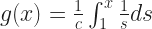

 but we already have
  in the works here. There is a limit to how many little one-stroke superscripts we need above g. This is the tradeoff to using ‘ for first derivatives. But here’s the important thing:


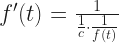


 for the correct value of c. Then all you need do is find a value of ‘c’ that makes that last equation true.
  . What is its velocity? That’s the first derivative of its position, so,
  .
.  is too small to notice. The motion declines into imperceptibility.
  , where
  .
.  , where
  and
and  are some real numbers whose value I don’t care about. What’s important here is that
  .
. 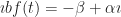 . This is an interesting complex number. Do you see what’s interesting about it? I’ll get there next paragraph.
  and
and  and
and  will all be
  for some real numbers a and b. In this case, you get spirals as t changes. If a is positive, you get points spiralling outward as t increases. If a is negative, you get points spiralling inward toward zero as t increases. If b is positive the spirals go counterclockwise. If b is negative the spirals go clockwise.
  is the same as
  .
.  , is equal to the product of the exponential of those terms. This is a good thing to have in your portfolio. If I remember right, it comes in around the 25th thing. It’s an easy result to have if you already showed something about the logarithms of products.
 then we get into tricky stuff. One response is to leave the answer like that:


 for ever-larger real numbers ‘x’. (This is the toy-compound-interest problem Bernoulli found.) But you can find the number other ways. You can calculate it — if you have the stamina — by working out the value of

 then we can find
  . The calculation on the right-hand side of this is easy; double your number and subtract one. Then to the lookup table; find the angle whose cosine is that number. That angle is two times θ. So divide that angle in two. Cosine of that is, well,

 . Or the cube of the sine of theta, or the cube of the tangent of theta. Whatever. The trouble is I don’t see a way to calculate cosine (sine, tangent) of 3θ, or 3 times the cosine (etc) of θ. Nor to get some other simple expression out of that. I can get mixtures of the cosine of 3θ plus the cosine of θ, sure. But that doesn’t help me figure out what θ is.
 instead. But if you don’t have a log table, and only have a table of cosines, you can calculate
  at least.


 it’s permitted, and common, to write it as
  . This means the same thing. I like that because, to me at least, it more clearly suggests “do this thing (take the second derivative) to the function we call ‘y’.” That’s a matter of style and what the author thinks needs emphasis.
  true. They all belong to one family, though. They all look like
  , where ‘C’ and ‘D’ are some fixed numbers. There’s no way to know, from what Lois has given, what those numbers should be. It might be that the context of the problem gives information to use to say what those numbers should be. It might be that the problem doesn’t care what those numbers should be. Impossible to say without the context.
 et cetera. There’s one step in it — “integration by parts” — that you’ll have to remember from freshman calculus, or maybe I’ll get around to explaining that someday, but I would expect most folks reading this far could follow this neat result.

 ? And if you can work that out, what about the number
  ?
? 
 .
. 
 or 0.16613. Multiply this by the logarithm of e (about 0.43429) and we have a common logarithm of about 0.07214. (We have an error estimate, too: we’ve got the natural logarithm of 1.1807 within a margin of error of
  , or about 0.000 0058, which, multiplied by the logarithm of e, corresponds to a margin of error for the common logarithm of about 0.000 0025.
 which is approximately 0.40729. If we were to work out the next term in the series, that would be
  , which has an absolute value of about 0.0026. So the natural logarithm of 1.5 is 0.40729, plus or minus 0.0026. If we only need the natural logarithm to within 0.0026, that’s good: we’re done.
  ; if I'm not mistaken, that's eight. Just how many terms we have to calculate will depend on what h is; the bigger it is — the farther the number is from 1 — the more terms we'll need.
 . That is, it’s not a difficult thing to write about, but it’s hard to find the audience for this number. It’s quite important, mathematically, but it hasn’t got an easy-to-understand definition like pi’s “the circumference of a circle divided by its diameter”. E’s most concise definition, I guess, is “the base of the natural logarithm”, which as an explanation to someone who hasn’t done much mathematics is only marginally more enlightening than slapping him with a slice of cold pizza. And it hasn’t got the sort of renown of something like the golden ratio which makes the number sound familiar and even welcoming.