From my Second A-to-Z: Orthonormal

For early 2016 — dubbed “Leap Day 2016” as that’s when it started — I got a request to explain orthogonal. I went in a different direction, although not completely different. This essay does get a bit more into specifics of how mathematicians use the idea, like, showing some calculations and such. I put in a casual description of vectors here. For book publication I’d want to rewrite that to be clearer that, like, ordered sets of numbers are just one (very common) way to represent vectors.

Jacob Kanev had requested “orthogonal” for this glossary. I’d be happy to oblige. But I used the word in last summer’s Mathematics A To Z. And I admit I’m tempted to just reprint that essay, since it would save some needed time. But I can do something more.

Orthonormal.

“Orthogonal” is another word for “perpendicular”. Mathematicians use it for reasons I’m not precisely sure of. My belief is that it’s because “perpendicular” sounds like we’re talking about directions. And we want to extend the idea to things that aren’t necessarily directions. As majors, mathematicians learn orthogonality for vectors, things pointing in different directions. Then we extend it to other ideas. To functions, particularly, but we can also define it for spaces and for other stuff.

I was vague, last summer, about how we do that. We do it by creating a function called the “inner product”. That takes in two of whatever things we’re measuring and gives us a real number. If the inner product of two things is zero, then the two things are orthogonal.

The first example mathematics majors learn of this, before they even hear the words “inner product”, are dot products. These are for vectors, ordered sets of numbers. The dot product we find by matching up numbers in the corresponding slots for the two vectors, multiplying them together, and then adding up the products. For example. Give me the vector with values (1, 2, 3), and the other vector with values (-6, 5, -4). The inner product will be 1 times -6 (which is -6) plus 2 times 5 (which is 10) plus 3 times -4 (which is -12). So that’s -6 + 10 – 12 or -8.

So those vectors aren’t orthogonal. But how about the vectors (1, -1, 0) and (0, 0, 1)? Their dot product is 1 times 0 (which is 0) plus -1 times 0 (which is 0) plus 0 times 1 (which is 0). The vectors are perpendicular. And if you tried drawing this you’d see, yeah, they are. The first vector we’d draw as being inside a flat plane, and the second vector as pointing up, through that plane, like a thumbtack.

So that’s orthogonal. What about this orthonormal stuff?

Well … the inner product can tell us something besides orthogonality. What happens if we take the inner product of a vector with itself? Say, (1, 2, 3) with itself? That’s going to be 1 times 1 (which is 1) plus 2 times 2 (4, according to rumor) plus 3 times 3 (which is 9). That’s 14, a tidy sum, although, so what?

The inner product of (-6, 5, -4) with itself? Oh, that’s some ugly numbers. Let’s skip it. How about the inner product of (1, -1, 0) with itself? That’ll be 1 times 1 (which is 1) plus -1 times -1 (which is positive 1) plus 0 times 0 (which is 0). That adds up to 2. And now, wait a minute. This might be something.

Start from somewhere. Move 1 unit to the east. (Don’t care what the unit is. Inches, kilometers, astronomical units, anything.) Then move -1 units to the north, or like normal people would say, 1 unit o the south. How far are you from the starting point? … Well, you’re the square root of 2 units away.

Now imagine starting from somewhere and moving 1 unit east, and then 2 units north, and then 3 units straight up, because you found a convenient elevator. How far are you from the starting point? This may take a moment of fiddling around with the Pythagorean theorem. But you’re the square root of 14 units away.

And what the heck, (0, 0, 1). The inner product of that with itself is 0 times 0 (which is zero) plus 0 times 0 (still zero) plus 1 times 1 (which is 1). That adds up to 1. And, yeah, if we go one unit straight up, we’re one unit away from where we started.

The inner product of a vector with itself gives us the square of the vector’s length. At least if we aren’t using some freak definition of inner products and lengths and vectors. And this is great! It means we can talk about the length — maybe better to say the size — of things that maybe don’t have obvious sizes.

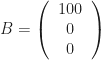
Some stuff will have convenient sizes. For example, they’ll have size 1. The vector (0, 0, 1) was one such. So is (1, 0, 0). And you can think of another example easily. Yes, it’s $\left(\frac{1}{\sqrt{2}}, -\frac{1}{2}, \frac{1}{2}\right)$ . (Go ahead, check!)

So by “orthonormal” we mean a collection of things that are orthogonal to each other, and that themselves are all of size 1. It’s a description of both what things are by themselves and how they relate to one another. A thing can’t be orthonormal by itself, for the same reason a line can’t be perpendicular to nothing in particular. But a pair of things might be orthogonal, and they might be the right length to be orthonormal too.

Why do this? Well, the same reasons we always do this. We can impose something like direction onto a problem. We might be able to break up a problem into simpler problems, one in each direction. We might at least be able to simplify the ways different directions are entangled. We might be able to write a problem’s solution as the sum of solutions to a standard set of representative simple problems. This one turns up all the time. And an orthogonal set of something is often a really good choice of a standard set of representative problems.

This sort of thing turns up a lot when solving differential equations. And those often turn up when we want to describe things that happen in the real world. So a good number of mathematicians develop a habit of looking for orthonormal sets.

My All 2020 Mathematics A to Z: Velocity

I’m happy to be back with long-form pieces. This week’s is another topic suggested by Mr Wu, of the Singapore Maths Tuition blog.

Color cartoon illustration of a coati in a beret and neckerchief, holding up a director's megaphone and looking over the Hollywood hills. The megaphone has the symbols + x (division obelus) and = on it. The Hollywood sign is, instead, the letters MATHEMATICS. In the background are spotlights, with several of them crossing so as to make the letters A and Z; one leg of the spotlights has 'TO' in it, so the art reads out, subtly, 'Mathematics A to Z'. — Art by Thomas K Dye, creator of the web comics **Projection Edge**, **Newshounds**, **Infinity Refugees**, and **Something Happens**. He’s on Twitter as @projectionedge. You can get to read **Projection Edge** six months early by subscribing to his Patreon.

Velocity.

This is easy. The velocity is the first derivative of the position. First derivative with respect to time, if you must know. That hardly needed an extra week to write.

Yes, there’s more. There is always more. Velocity is important by itself. It’s also important for guiding us into new ideas. There are many. One idea is that it’s often the first good example of vectors. Many things can be vectors, as mathematicians see them. But the ones we think of most often are “some magnitude, in some direction”.

The position of things, in space, we describe with vectors. But somehow velocity, the changes of positions, seems more significant. I suspect we often find static things below our interest. I remember as a physics major that my Intro to Mechanics instructor skipped Statics altogether. There are many important things, like bridges and roofs and roller coaster supports, that we find interesting because they don’t move. But the real Intro to Mechanics is stuff in motion. Balls rolling down inclined planes. Pendulums. Blocks on springs. Also planets. (And bridges and roofs and roller coaster supports wouldn’t work if they didn’t move a bit. It’s not much though.)

So velocity shows us vectors. Anything could, in principle, be moving in any direction, with any speed. We can imagine a thing in motion inside a room that’s in motion, its net velocity being the sum of two vectors.

And they show us derivatives. A compelling answer to “what does differentiation mean?” is “it’s the rate at which something changes”. Properly, we can take the derivative of any quantity with respect to any variable. But there are some that make sense to do, and position with respect to time is one. Anyone who’s tried to catch a ball understands the interest in knowing.

We take derivatives with respect to time so often we have shorthands for it, by putting a ‘ mark after, or a dot above, the variable. So if x is the position (and it often is), then $x'$ is the velocity. If we want to emphasize we think of vectors, $\vec{x}$ is the position and $\vec{x}'$ the velocity.

Velocity has another common shorthand. This is $v$ , or if we want to emphasize its vector nature, $\vec{v}$ . Why a name besides the good enough $\vec{x}'$ ? It helps us avoid misplacing a ‘ mark in our work, for one. And giving velocity a separate symbol encourages us to think of the velocity as independent from the position. It’s not — not exactly — independent. But knowing that a thing is in the lawn outside tells us nothing about how it’s moving. Velocity affects position, in a process so familiar we rarely consider how there’s parts we don’t understand about it. But velocity is also somehow also free of the position at an instant.

Velocity also guides us into a first understanding of how to take derivatives. Thinking of the change in position over smaller and smaller time intervals gets us to the “instantaneous” velocity by doing only things we can imagine doing with a ruler and a stopwatch.

Velocity has a velocity. $\vec{v}'$ , also known as $\vec{a}$ . Or, if we’re sure we won’t lose a ‘ mark, $\vec{x}''$ . Once we are comfortable thinking of how position changes in time we can think of other changes. Velocity’s change in time we call acceleration. This is also a vector, more abstract than position or velocity. Multiply the acceleration by the mass of the thing accelerating and we have a vector called the “force”. That, we at least feel we understand, and can work with.

Acceleration has a velocity too, a rate of change in time. It’s called the “jerk” by people telling you the change in acceleration in time is called the “jerk”. (I don’t see the term used in the wild, but admit my experience is limited.) And so on. We could, in principle, keep taking derivatives of the position and keep finding new changes. But most physics problems we find interesting use just a couple of derivatives of the position. We can label them, if we need, $\vec{x}^{(n)}$ , where n is some big enough number like 4.

We can bundle them in interesting ways, though. Come back to that mention of treating position and velocity of something as though they were independent coordinates. It’s a useful perspective. Imagine the rules about how particles interacting with one another and with their environment. These usually have explicit roles for position and velocity. (Granting this may reflect a selection bias. But these do cover enough interesting problems to fill a career.)

So we create a new vector. It’s made of the positition and the velocity. We’d write it out as $(x, v)^T$ . The superscript-T there, “transposition”, lets us use the tools of matrix algebra. This vector describes a point in phase space. Phase space is the collection of all the physically possible positions and velocities for the system.

What’s the derivative, in time, of this point in phase space? Glad to say we can do this piece by piece. The derivative of a vector is the derivative of each component of a vector. So the derivative of $(x, v)^T$ is $(x', v')^T$ , or, $(v, a)^T$ . This acceleration itself depends on, normally, the positions and velocities. So we can describe this as $(v, f(x, v))^T$ for some function $f(x, v)$ . You are surely impressed with this symbol-shuffling. You are less sure why this bother.

The bother is a trick of ordinary differential equations. All differential equations are about how a function-to-be-determined and its derivatives relate to one another. In ordinary differential equations, the function-to-be-determined depends on a single variable. Usually it’s called x or t. There may be many derivatives of f. This symbol-shuffling rewriting takes away those higher-order derivatives. We rewrite the equation as a vector equation of just one order. There’s some point in phase space, and we know what its velocity is. That we do because in this form many problems can be written as a matrix problem: $\vec{x}' = A\vec{x}$ . Or approximate our problem as a matrix problem. This lets us bring in linear algebra tools, and that’s worthwhile.

It also lets us bring in numerical tools. Numerical mathematics has developed many methods to solve the ordinary differential equation $x' = f(x)$ . Most of them extend to $\vec{x}' = f(\vec{x})$ . The result is a classic mathematician’s trick. We can recast a problem as one we have better tools to solve.

It calls on a more abstract idea of what a “velocity” might be. We can explain what the thing that’s “moving” and what it’s moving through are, given time. But the instincts we develop from watching ordinary things move help us in these new territories. This is also a classic mathematician’s trick. It may seem like all mathematicians do is develop tricks to extend what they already do. I can’t say this is wrong.

Thank you all for reading and for putting up with my gap week. This and all of my 2020 A-to-Z essays should be at this link. All the essays from every A-to-Z series should be at this link.

My All 2020 Mathematics A to Z: J Willard Gibbs

Charles Merritt sugested a biographical subject for G. (There are often running themes in an A-to-Z and this year’s seems to be “biography”.) I don’t know of a web site or other project that Merritt has that’s worth sharing, but if I learn of it, I’ll pass it along.

J Willard Gibbs.

My love and I, like many people, tried last week to see the comet NEOWISE. It took several attempts. When finally we had binoculars and dark enough sky we still had the challenge of where to look. Finally determined searching and peripheral vision (which is more sensitive to faint objects) found the comet. But how to guide the other to a thing barely visible except with binoculars? Between the silhouettes of trees and a convenient pair of guide stars we were able to put the comet’s approximate location in words. Soon we were experts at finding it. We could turn a head, hold up the binoculars, and see a blue-ish puff of something.

To perceive a thing is not to see it. Astronomy is full of things seen but not recognized as important. There is a great need for people who can describe to us how to see a thing. And this is part of the significance of J Willard Gibbs.

American science, in the 19th century, had an inferiority complex compared to European science. Fairly, to an extent: what great thinkers did the United States have to compare to William Thompson or Joseph Fourier or James Clerk Maxwell? The United States tried to argue that its thinkers were more practical minded, with Joseph Henry as example. Without downplaying Henry’s work, though? The stories of his meeting the great minds of Europe are about how he could fix gear that Michael Faraday could not. There is a genius in this, yes. But we are more impressed by magnetic fields than by any electromagnet.

Gibbs is the era’s exception, a mathematical physicist of rare insight and creativity. In his ability to understand problems, yes. But also in organizing ways to look at problems so others can understand them better. A good comparison is to Richard Feynman, who understood a great variety of problems, and organized them for other people to understand. No one, then or now, doubted Gibbs compared well to the best European minds.

Gibbs’s life story is almost the type case for a quiet academic life. He was born into an academic/ministerial family. Attended Yale. Earned what appears to be the first PhD in engineering granted in the United States, and only the fifth non-honorary PhD in the country. Went to Europe for three years, then came back home, got a position teaching at Yale, and never left again. He was appointed Professor of Mathematical Physics, the first such in the country, at age 32 and before he had even published anything. This speaks of how well-connected his family was. Also that he was well-off enough not to need a salary. He wouldn’t take one until 1880, when Yale offered him two thousand per year against Johns Hopkins’s three.

Between taking his job and taking his salary, Gibbs took time to remake physics. This was in thermodynamics, possibly the most vibrant field of 19th century physics. The wonder and excitement we see in quantum mechanics resided in thermodynamics back then. Though with the difference that people with a lot of money were quite interested in the field’s results. These were people who owned railroads, or factories, or traction companies. Extremely practical fields.

What Gibbs offered was space, particularly, phase space. Phase space describes the state of a system as a point in … space. The evolution of a system is typically a path winding through space. Constraints, like the conservation of energy, we can usually understand as fixing the system to a surface in phase space. Phase space can be as simple as “the positions and momentums of every particle”, and that often is what we use. It doesn’t need to be, though. Gibbs put out diagrams where the coordinates were things like temperature or pressure or entropy or energy. Looking at these can let one understand a thermodynamic system. They use our geometric sense much the same way that charts of high- and low-pressure fronts let one understand the weather. James Clerk Maxwell, famous for electromagnetism, was so taken by this he created plaster models of the described surface.

This is, you might imagine, pretty serious, heady stuff. So you get why Gibbs published it in the Transactions of the Connecticut Academy: his brother-in-law was the editor. It did not give the journal lasting fame. It gave his brother-in-law a heightened typesetting bill, and Yale faculty and New Haven businessmen donated funds.

Which gets to the less-happy parts of Gibbs’s career. (I started out with ‘less pleasant’ but it’s hard to spot an actually unpleasant part of his career.) This work sank without a trace, despite Maxwell’s enthusiasm. It emerged only in the middle of the 20th century, as physicists came to understand their field as an expression of geometry.

That’s all right. Chemists understood the value of Gibbs’s thermodynamics work. He introduced the enthalpy, an important thing that nobody with less than a Master’s degree in Physics feels they understand. Changes of enthalpy describe how heat transfers. And the Gibbs Free Energy, which measures how much reversible work a system can do if the temperature and pressure stay constant. A chemical reaction where the Gibbs free energy is negative will happen spontaneously. If the system’s in equilibrium, the Gibbs free energy won’t change. (I need to say the Gibbs free energy as there’s a different quantity, the Helmholtz free energy, that’s also important but not the same thing.) And, from this, the phase rule. That describes how many independently-controllable variables you can see in mixing substances.

In the 1880s Gibbs worked on something which exploded through physics and mathematics. This was vectors. He didn’t create them from nothing. Hermann Günter Grassmann — whose fascinating and frustrating career I hadn’t known of before this — laid much of the foundation. Building on Grassman and W K Clifford, though, let Gibbs present vectors as we now use them in physics. How to define dot products and cross products. How to use them to simplify physics problems. How they’re less work than quaternions are. Gibbs was not the only person to recast physics in vector form. Oliver Heaviside is another important mathematical physicist of the time who did. But Gibbs identified the tools extremely well. You can read his Elements of Vector Analysis. It’s not very different from what a modern author would write on the subject. It’s terser than I would write, but terse is also respectful of someone’s time and ability to reason out explanations of small points.

There are more pieces. They don’t all fit in a neat linear timeline; nobody’s life really does. Gibbs’s thermodynamics work, leading into statistical mechanics, foreshadows much of quantum mechanics. He’s famous for the Gibbs Paradox, which concerns the entropy of mixing together two different kinds of gas. Why is this different from mixing together two containers of the same kind of gas? And the answer is that we have to think more carefully about what we mean by entropy, and about the differences between containers.

There is a Gibbs phenomenon, known to anyone studying Fourier series. The Fourier series is a sum of sine and cosine functions. It approximates an arbitrary original function. The series is a continuous function; you could draw it without lifting your pen. If the original function has a jump, though? A spot where you have to lift your pen? The Fourier series for that represents the jump with a region where its quite-good approximation suddenly turns bad. It wobbles around the ‘correct’ values near the jump. Using more terms in the series doesn’t make the wobbling shrink. Gibbs described it, in studying sawtooth waves. As it happens, Henry Wilbraham first noticed and described this in 1848. But Wilbraham’s work went unnoticed until after Gibbs’s rediscovery.

And then there was a bit in which Gibbs was intrigued by a comet that prolific comet-spotter Lewis Swift observed in 1880. Finding the orbit of a thing from a handful of observations is one of the great problems of astronomical mathematics. Karl Friedrich Gauss started the 19th century with his work projecting the orbit of the newly-discovered and rapidly-lost asteroid Ceres. Gibbs put his vector notation to the work of calculating orbits. His technique, I am told by people who seem to know, is less difficult and more numerically stable than was earlier used.

Swift’s comet of 1880, it turns out, was spotted in 1869 by Wilhelm Tempel. It was lost after its 1908 perihelion. Comets have a nasty habit of changing their orbits on us. But it was rediscovered in 2001 by the Lincoln Near-Earth Asteroid Research program. It’s next to reach perihelion the 26th of November, 2020. You might get to see this, another thing touched by J Willard Gibbs.

This and the other other A-to-Z topics for 2020 should be at this link. All my essays for this and past A-to-Z sequences are at this link. I’ll soon be opening f or topics for J, K, and L, essays also. Thanks for reading.

My 2019 Mathematics A To Z: Norm

Today’s A To Z term is another free choice. So I’m picking a term from the world of … mathematics. There are a lot of norms out there. Many are specialized to particular roles, such as looking at complex-valued numbers, or vectors, or matrices, or polynomials.

Still they share things in common, and that’s what this essay is for. And I’ve brushed up against the topic before.

The norm, also, has nothing particular to do with “normal”. “Normal” is an adjective which attaches to every noun in mathematics. This is security for me as while these A-To-Z sequences may run out of X and Y and W letters, I will never be short of N’s.

Cartoony banner illustration of a coati, a raccoon-like animal, flying a kite in the clear autumn sky. A skywriting plane has written 'MATHEMATIC A TO Z'; the kite, with the letter 'S' on it to make the word 'MATHEMATICS'. — Art by Thomas K Dye, creator of the web comics **Projection Edge**, **Newshounds**, **Infinity Refugees**, and **Something Happens**. He’s on Twitter as @projectionedge. You can get to read **Projection Edge** six months early by subscribing to his Patreon.

Norm.

A “norm” is the size of whatever kind of thing you’re working with. You can see where this is something we look for. It’s easy to look at two things and wonder which is the smaller.

There are many norms, even for one set of things. Some seem compelling. For the real numbers, we usually let the absolute value do this work. By “usually” I mean “I don’t remember ever seeing a different one except from someone introducing the idea of other norms”. For a complex-valued number, it’s usually the square root of the sum of the square of the real part and the square of the imaginary coefficient. For a vector, it’s usually the square root of the vector dot-product with itself. (Dot product is this binary operation that is like multiplication, if you squint, for vectors.) Again, these, the “usually” means “always except when someone’s trying to make a point”.

Which is why we have the convention that there is a “the norm” for a kind of operation. The norm dignified as “the” is usually the one that looks as much as possible like the way we find distances between two points on a plane. I assume this is because we bring our intuition about everyday geometry to mathematical structures. You know how it is. Given an infinity of possible choices we take the one that seems least difficult.

Every sort of thing which can have a norm, that I can think of, is a vector space. This might be my failing imagination. It may also be that it’s quite easy to have a vector space. A vector space is a collection of things with some rules. Those rules are about adding the things inside the vector space, and multiplying the things in the vector space by scalars. These rules are not difficult requirements to meet. So a lot of mathematical structures are vector spaces, and the things inside them are vectors.

A norm is a function that has these vectors as its domain, and the non-negative real numbers as its range. And there are three rules that it has to meet. So. Give me a vector ‘u’ and a vector ‘v’. I’ll also need a scalar, ‘a. Then the function f is a norm when:

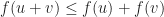$f(u + v) \le f(u) + f(v)$ . This is a famous rule, called the triangle inequality. You know how in a triangle, the sum of the lengths of any two legs is greater than the length of the third leg? That’s the rule at work here.
$f(a\cdot u) = |a| \cdot f(u)$ . This doesn’t have so snappy a name. Sorry. It’s something about being homogeneous, at least.
If $f(u) = 0$ then u has to be the additive identity, the vector that works like zero does.

Norms take on many shapes. They depend on the kind of thing we measure, and what we find interesting about those things. Some are familiar. Look at a Euclidean space, with Cartesian coordinates, so that we might write something like (3, 4) to describe a point. The “the norm” for this, called the Euclidean norm or the L² norm, is the square root of the sum of the squares of the coordinates. So, 5. But there are other norms. The L¹ norm is the sum of the absolute values of all the coefficients; here, 7. The L^∞ norm is the largest single absolute value of any coefficient; here, 4.

A polynomial, meanwhile? Write it out as $a_0 + a_1 x + a_2 x^2 + a_3 x^3 + \cdots + a_n x^n$ . Take the absolute value of each of these $a_k$ terms. Then … you have choices. You could take those absolute values and add them up. That’s the L¹ polynomial norm. Take those absolute values and square them, then add those squares, and take the square root of that sum. That’s the L² norm. Take the largest absolute value of any of these coefficients. That’s the L^∞ norm.

These don’t look so different, even though points in space and polynomials seem to be different things. We designed the tool. We want it not to be weirder than it has to be. When we try to put a norm on a new kind of thing, we look for a norm that resembles the old kind of thing. For example, when we want to define the norm of a matrix, we’ll typically rely on a norm we’ve already found for a vector. At least to set up the matrix norm; in practice, we might do a calculation that doesn’t explicitly use a vector’s norm, but gives us the same answer.

If we have a norm for some vector space, then we have an idea of distance. We can say how far apart two vectors are. It’s the norm of the difference between the vectors. This is called defining a metric on the vector space. A metric is that sense of how far apart two things are. What keeps a norm and a metric from being the same thing is that it’s possible to come up with a metric that doesn’t match any sensible norm.

It’s always possible to use a norm to define a metric, though. Doing that promotes our normed vector space to the dignified status of a “metric space”. Many of the spaces we find interesting enough to work in are such metric spaces. It’s hard to think of doing without some idea of size.

I’ve made it through one more week without missing deadline! This and all the other Fall 2019 A To Z posts should be at this link. I remain open for subjects for the letters Q through T, and would appreciate nominations at this link. Thank you for reading and I’ll fill out the rest of this week with reminders of old A-to-Z essays.

Reading the Comics, August 31, 2019: Martin V Edition

And so the Reading the Comics posts have returned to Sunday after a month in exile to Tuesdays. I’m curious whether Sunday is actually the best day to post my signature series of essays, since everybody is usually doing stuff on the weekends. Tuesdays more people are at work and looking for other things to think about. But at least for the duration of the A to Z series there’s not a good time to schedule them besides Sundays. So Sundays it is and I’ll possibly think things over again in December, if all goes well.

Ralph Hagen’s The Barn for the 27th poses a question that’s ridiculous when you look at it. Why should being twenty times as old as your newborn (sic) when you’re twenty years old imply you’d be twenty times as old as the newborn when you’re sixty? Age increases linearly. The ratios between ages, though, those decrease, in a ratio asymptotically approaching 1. So as far as that goes, this strip isn’t much of anything.

Rory, sheep: 'How come if you're 20 when our child is born, you're 20 times older when your child is born, but by the time you're 60, you're only 1.5 times older?' (Rory leaves.) Stan, cow: 'Did you order a math puzzle?' Karl, frog: 'Nope. Cheese pizza, extra flies.' — Ralph Hagen’s **The Barn** for the 27th of August, 2019. I was wondering if this might be a new tag. It’s not. Other essays featuring **The Barn** are at this link.

But I do like how it captures the way a mathematics puzzle can come from nowhere. Often interesting ones seem to generate themselves. You notice a pattern and wonder whether it reaches some interesting point. If you convince yourself it does, you wonder when it does. If it does not, you wonder why it can’t. This is the fun sort of mathematics, and you create it by looking at the two separate tile patterns in the kitchen or, as here, thinking about the ages of parent and child. Anything that catches the imagination of a bored mind. It’s fun being there.

Rory (the sheep) makes a common enough slip. Saying a twenty-year-old with a newborn is twenty times as old as the newborn is, implicitly, saying the newborn is one year old. This kind of error is so common it’s got a folksy name, the “fencepost error”. It has a more respectable name, for its LinkedIn profile, the “off-by-one error”. But you see the problem. Say that your birthday is the 1st of September. How many times were you alive on the 1st of September by the time you’re ten years old? Eleven times, the first one being the one you were born on, with one more counted up each year you’d lived. This was probably more clear before I explained it.

Teacher: 'You deserve an 'A' for your creative writing, Jughaid. But this is 'rithmetic!!' On the blackboard Jughead's written out 2 + 4 = 10, 6 + 5 = 7, 8 + 3 = 15, 7 + 1 = 5, 9 + 4 = 23. — John Rose’s **Barney Google and Snuffy Smith** for the 27th of August, 2019. This one I kept finding when I was looking for **The Barn**. Essays based on something raised by **Barney Google** should be at this link.

John Rose’s Barney Google and Snuffy Smith for the 27th has Mis Prunelly complimenting Jughaid’s creativity, but not wanting it in arithmetic. There is creativity in mathematics. And there is great value in calculating something in an original way. There’s value in calculating things wrong, too, if it’s an approximate calculation. Knowing whether your answer is nearer 10 or 20 is of some value, and it might be all that you in fact want. That’s being wrong in a productive way, though.

Harry Bliss and Steve Martin’s Bliss for the 27th uses a string of mathematical symbols as emblem of genius. Most of the symbols look just near enough meaningful that I wonder if Bliss and Martin got a mathematician friend of theirs to give them some scraps. Why I say mathematician rather than, say, physicist is because some of the lines look more mathematician than physicist.

Illustrated book cover: 'They Called Me Dumbo: A Memoir of Redemption'. Dumbo's shown in front of Princeton, and writing a column of arithmetic using a pencil held by his trunk. — Harry Bliss and Steve Martin’s **Bliss** for the 27th of August, 2019. Essays that do feature **Bliss** should be gathered at this link.

The most distinctive one, to me, is right above Dumbo’s pencil and trunk there: $g^{-1}\cdot g = e$ . This is the kind of equation you’ll see all the time in group theory. It’s an important field of mathematics, the one studying sets that work like arithmetic does. This starts with groups, which have a set of things and a binary operation between those things. Think of it as either addition or multiplication. You notice that $g^{-1} \cdot g = e$ already looks like multiplication. ‘g’ and ‘h’ serve, for group theory, the roles that ‘x’ and ‘y’ do in (high school) algebra. ‘x’ and ‘y’ mean some number, whose value we might or might not care about. Similarly, ‘g’ and ‘h’ are some elements, things in the set for our group. We might or might not care which ones they are. $e$ means the identity element, the thing which won’t change the value of the other partner in an operation. The thing that works like zero for addition, or like one for multiplication. And $g^{-1}$ means the inverse of $g$ : the thing which, added (or multiplied) to $g$ gives us the identity element. So if we were talking addition and $g$ were 5, then $g^{-1}$ would be -5. This might not sound like very much, but we can make it complicated.

Also distinctive to me: that first line. I’m not perfectly sure I’m transcribing this right. But it looks a good deal to me like the binomial distribution. This is the probability of seeing something happen k times, if you give it n chances to happen, and every chance has the same probability p of it happening. The formula isn’t quite right. It’s missing a power on the (1 – p) term at the end. But it’s wrong in ways that make sense for the need to draw something legible.

Just under Dumbo’s pencil, too, is a line that I had to look up how to render in WordPress’s LaTeX. It’s the one about $\left| X \cup Y \right| = \left| X \right| + \left| Y \right|$ . The union symbol, the U there, speaks of set theory. It means to form a new set, one that has all the elements in the set called X or the set called Y or both. The straight vertical lines flanking these set names or descriptions are how we describe taking the norm, finding the size, of a set. This is ordinarily how many things are inside the set. If the sets X and Y have no elements in common, then the size of the union of X and Y will be the size of the set X plus the size of the set Y.

There’s other lines that come near making sense. The line about $f : x \rightarrow xnW$ has the form of the “mapping” way to define a function. I just don’t understand what the rule here means. The final line, $= e \frac{-t^2}{2} !$ , first … well, this sort of e-raised-to-the-minus-something-squared form turns up all the time. But second, to end a bit of work with an exclamation point really captures the surprise and joy of having reached a goal. Mathematicians take delight in their work, like you’d expect.

A 'solved' Rubik's cube sits on the left. On the right a scrambled cube, with one row of the top face a quarter-turn out of place, says, 'Some days are better than others.' — Maria Scrivan’s **Half Full** for the 29th of August, 2019. Other appearances by **Half Full** should be behind this link.

Maria Scrivan’s Half Full for the 29th is a Rubik’s Cube joke. A variation of it ran back in June 2018. I hate that this time I noticed that on the right, the cubelet — with white on top, red on the lower left, and green on the lower right — is inconsistent with the ordered cube. The corresponding cubelet there has blue on top, red on the lower left, and green on the lower right. Well, maybe the cube on the right had its color stickers applied differently. This is a little thing. But it’s close to a problem that turns up all the time in representing geometry. It’s easy to say you have, say, axes going in the x, y, and z directions. But which direction is x? Which is y? Which is z? You can lay all three out so every pair makes a right angle. Whatever way you lay them out will turn out to be, up to a rotation, one of two patterns. Let’s say the x axis points east, and the y axis points north. Then the z axis can point up. Or it can point down. You can pick which one makes sense for your problem. The two choices are mirror images of the other. You get primed to notice this when you do mathematical physics. The Rubik’s Cube on the left is just this kind of representation, with (let’s say) the red face pointing in the x direction, the green face pointing in the y direction, and the blue pointing in the z direction. Which is a lot of thought to put into what was an arbitrary choice, as I’m sure the cartoonist (or whoever did the coloring) just wanted a cube that looked attractive.

There were a surprising number of comics that mentioned mathematics, but not enough for a paragraph. I’ll feature them in another essay run here sometime this week. Also starting this week: the Fall 2019 Mathematics A To Z. It’s still not too late to suggest topics for the letters C through H!

In Which I Offer Excuses Instead Of Mathematics

I’d been hoping to get back into longer-form essays. And then the calculations I meant to do on one problem turned out more complicated than I’d wanted. And they’re hard to square with the approach I used in some earlier work. Not that the results I was looking at were wrong, mind, just that an approach I’d used as “convenient for this sort of problem” turned inconvenient here.

So while I have the whole piece back in the shop for re-thinking, which is harder than even thinking, let me give you some other stuff to read. Or look at. One is from regular Singaporean correspondent MathTuition88. If you know anything about topology it’s because you’ve heard about Möbius strips. Surfaces with a single side are neat, and form the base of 95 percent of all science fiction stories in which the mathematics is the fantastic element. Klein bottles are often mentioned as a four-dimensional analogue to the Möbius strip, a solid object with no distinguishable interior or exterior. And a Klein bottle can be divided into two Möbius strips. MathTuition88 showcases a picture about how to turn two strips into a bottle. Or at least the best approximation of a bottle we can do; the actual Klein bottle is a four-dimensional structure and we can just make a three-dimensional imitation of the thing.

For something a bit more vector-analytic Joe Heafner’s Tensor Time has an essay about vectors. It’s about Heafner’s dislike for the way some vector problems are presented. Some common and easy ways to solve vector equations lead to spurious solutions that have to be weeded out by ad hoc reasoning; can’t we do better? Heafner argues that we can and should. The suggested alternative looks a little stuffy, but as often happens, spending more time on the setup means one spends less time confused later on. Worth pondering.

And this is a late addition, but I couldn’t resist.

Just found this gem : "Calculus Made Easy" (1910). Oh why didn't my high-school book start with ch. 1?!
Full pdf: https://t.co/usC2TDpvW7 pic.twitter.com/xFsQT1Y5RD

— Rasmus Bååth (@rabaath) April 20, 2017

Now I have a new favorite first chapter for a calculus text.

The End 2016 Mathematics A To Z: Hat

I was hoping to pick a term that was a quick and easy one to dash off. I learned better.

Hat.

This is a simple one. It’s about notation. Notation is never simple. But it’s important. Good symbols organize our thoughts. They tell us what are the common ordinary bits of our problem, and what are the unique bits we need to pay attention to here. We like them to be easy to write. Easy to type is nice, too, but in my experience mathematicians work by hand first. Typing is tidying-up, and we accept that being sluggish. Unique would be nice, so that anyone knows what kind of work we’re doing just by looking at the symbols. I don’t think anything manages that. But at least some notation has alternate uses rare enough we don’t have to worry about it.

“Hat” has two major uses I know of. And we call it “hat”, although our friends in the languages department would point out this is a caret. The little pointy corner that goes above a letter, like so: $\hat{i}$ . $\hat{x}$ . $\hat{e}$ . It’s not something we see on its own. It’s always above some variable.

The first use of the hat like this comes up in statistics. It’s a way of marking that something is an estimate. By “estimate” here we mean what anyone might mean by “estimate”. Statistics is full of uses for this sort of thing. For example, we often want to know what the arithmetic mean of some quantity is. The average height of people. The average temperature for the 18th of November. The average weight of a loaf of bread. We have some letter that we use to mean “the value this has for any one example”. By some letter we mean ‘x’, maybe sometimes ‘y’. We can use any and maybe the problem begs for something. But it’s ‘x’, maybe sometimes ‘y’.

For the arithmetic mean of ‘x’ for the whole population we write the letter with a horizontal bar over it. (The arithmetic mean is the thing everybody in the world except mathematicians calls the average. Also, it’s what mathematicians mean when they say the average. We just get fussy because we know if we don’t say “arithmetic mean” someone will come along and point out there are other averages.) That arithmetic mean is $\bar{x}$ . Maybe $\bar{y}$ if we must. Must be some number. But what is it? If we can’t measure whatever it is for every single example of our group — the whole population — then we have to make an estimate. We do that by taking a sample, ideally one that isn’t biased in some way. (This is so hard to do, or at least be sure you’ve done.) We can find the mean for this sample, though, because that’s how we picked it. The mean of this sample is probably close to the mean of the whole population. It’s an estimate. So we can write $\hat{x}$ and understand. This is not $\bar{x}$ but it does give us a good idea what $\hat{x}$ should be.

(We don’t always use the caret ^ for this. Sometimes we use a tilde ~ instead. ~ has the advantage that it’s often used for “approximately equal to”. So it will carry that suggestion over to its new context.)

The other major use of the hat comes in vectors. Mathematics types do a lot of work with vectors. It turns out a lot of mathematical structures work the way that pointing and moving in directions in ordinary space do. That’s why back when I talked about what vectors were I didn’t say “they’re like arrows pointing some length in some direction”. Arrows pointing some length in some direction are vectors, yes, but there are many more things that are vectors. Thinking of moving in particular directions gives us good intuition for how to work with vectors, and for stuff that turns out to be vectors. But they’re not everything.

If we need to highlight that something is a vector we put a little arrow over its name. $\vec{x}$ . $\vec{e}$ . That sort of thing. (Or if we’re typing, we might put the letter in boldface: x. This was good back before computers let us put in mathematics without giving the typesetters hazard pay.) We don’t always do that. By the time we do a lot of stuff with vectors we don’t always need the reminder. But we will include it if we need a warning. Like if we want to have both $\vec{r}$ telling us where something is and to use a plain old $r$ to tell us how big the vector $\vec{r}$ is. That turns up a lot in physics problems.

Every vector has some length. Even vectors that don’t seem to have anything to do with distances do. We can make a perfectly good vector out of “polynomials defined for the domain of numbers between -2 and +2”. Those polynomials are vectors, and they have lengths.

There’s a special class of vectors, ones that we really like in mathematics. They’re the “unit vectors”. Those are vectors with a length of 1. And we are always glad to see them. They’re usually good choices for a basis. Basis vectors are useful things. They give us, in a way, a representative slate of cases to solve. Then we can use that representative slate to give us whatever our specific problem’s solution is. So mathematicians learn to look instinctively to them. We want basis vectors, and we really like them to have a length of 1. Even if we aren’t putting the arrow over our variables we’ll put the caret over the unit vectors.

There are some unit vectors we use all the time. One is just the directions in space. That’s $\hat{e}_1$ and $\hat{e}_2$ and for that matter $\hat{e}_3$ and I bet you have an idea what the next one in the set might be. You might be right. These are basis vectors for normal, Euclidean space, which is why they’re labelled “e”. We have as many of them as we have dimensions of space. We have as many dimensions of space as we need for whatever problem we’re working on. If we need a basis vector and aren’t sure which one, we summon one of the letters used as indices all the time. $\hat{e}_i$ , say, or $\hat{e}_j$ . If we have an n-dimensional space, then we have unit vectors all the way up to $\hat{e}_n$ .

We also use the hat a lot if we’re writing quaternions. You remember quaternions, vaguely. They’re complex-valued numbers for people who’re bored with complex-valued numbers and want some thrills again. We build them as a quartet of numbers, each added together. Three of them are multiplied by the mysterious numbers ‘i’, ‘j’, and ‘k’. Each ‘i’, ‘j’, or ‘k’ multiplied by itself is equal to -1. But ‘i’ doesn’t equal ‘j’. Nor does ‘j’ equal ‘k’. Nor does ‘k’ equal ‘i’. And ‘i’ times ‘j’ is ‘k’, while ‘j’ times ‘i’ is minus ‘k’. That sort of thing. Easy to look up. You don’t need to know all the rules just now.

But we often end up writing a quaternion as a number like $4 + 2\hat{i} - 3\hat{j} + 1 \hat{k}$ . OK, that’s just the one number. But we will write numbers like 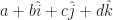$a + b\hat{i} + c\hat{j} + d\hat{k}$ . Here a, b, c, and d are all real numbers. This is kind of sloppy; the pieces of a quaternion aren’t in fact vectors added together. But it is hard not to look at a quaternion and see something pointing in some direction, like the first vectors we ever learn about. And there are some problems in pointing-in-a-direction vectors that quaternions handle so well. (Mostly how to rotate one direction around another axis.) So a bit of vector notation seeps in where it isn’t appropriate.

I suppose there’s some value in pointing out that the ‘i’ and ‘j’ and ‘k’ in a quaternion are fixed and set numbers. They’re unlike an ‘a’ or an ‘x’ we might see in the expression. I’m not sure anyone was thinking they were, though. Notation is a tricky thing. It’s as hard to get sensible and consistent and clear as it is to make words and grammar sensible. But the hat is a simple one. It’s good to have something like that to rely on.

Reading the Comics, September 24, 2016: Infinities Happen Edition

I admit it’s a weak theme. But two of the comics this week give me reason to talk about infinitely large things and how the fact of being infinitely large affects the probability of something happening. That’s enough for a mid-September week of comics.

Kieran Meehan’s Pros and Cons for the 18th of September is a lottery problem. There’s a fun bit of mathematical philosophy behind it. Supposing that a lottery runs long enough without changing its rules, and that it does draw its numbers randomly, it does seem to follow that any valid set of numbers will come up eventually. At least, the probability is 1 that the pre-selected set of numbers will come up if the lottery runs long enough. But that doesn’t mean it’s assured. There’s not any law, physical or logical, compelling every set of numbers to come up. But that is exactly akin to tossing a coin fairly infinity many times and having it come up tails every single time. There’s no reason that can’t happen, but it can’t happen.

'It's true, Dr Peel. I'm a bit of a psychic.' 'Would you share the winning lottery numbers with me?' '1, 10, 17, 39, 43, and 47'. 'Those are the winning lottery numbers?' 'Yes!' 'For this Tuesday?' 'Ah! That's where it gets a bit fuzzy.' — Kieran Meehan’s **Pros and Cons** for the 18th of September, 2016. I can’t say whether any of these are supposed to be the PowerBall number. (The comic strip’s title is a revision of its original, which more precisely described its gimmick but was harder to remember: **A Lawyer, A Doctor, and a Cop**.)

Leigh Rubin’s Rubes for the 19th name-drops chaos theory. It’s wordplay, as of course it is, since the mathematical chaos isn’t the confusion-and-panicky-disorder of the colloquial term. Mathematical chaos is about the bizarre idea that a system can follow exactly perfectly known rules, and yet still be impossible to predict. Henri Poincaré brought this disturbing possibility to mathematicians’ attention in the 1890s, in studying the question of whether the solar system is stable. But it lay mostly fallow until the 1960s when computers made it easy to work this out numerically and really see chaos unfold. The mathematician type in the drawing evokes Einstein without being too close to him, to my eye.

Allison Barrows’s PreTeena rerun of the 20th shows some motivated calculations. It’s always fun to see people getting excited over what a little multiplication can do. Multiplying a little change by a lot of chances is one of the ways to understanding integral calculus, and there’s much that’s thrilling in that. But cutting four hours a night of sleep is not a little thing and I wouldn’t advise it for anyone.

Jason Poland’s Robbie and Bobby for the 20th riffs on Jorge Luis Borges’s Library of Babel. It’s a great image, the idea of the library containing every book possible. And it’s good mathematics also; it’s a good way to probe one’s understanding of infinity and of probability. Probably logic, also. After all, grant that the index to the Library of Babel is a book, and therefore in the library somehow. How do you know you’ve found the index that hasn’t got any errors in it?

Ernie Bushmiller’s Nancy Classics for the 21st originally ran the 21st of September, 1949. It’s another example of arithmetic as a proof of intelligence. Routine example, although it’s crafted with the usual Bushmiller precision. Even the close-up, peering-into-your-soul image if Professor Stroodle in the second panel serves the joke; without it the stress on his wrinkled brow would be diffused. I can’t fault anyone not caring for the joke; it’s not much of one. But wow is the comic strip optimized to deliver it.

Thom Bluemel’s Birdbrains for the 23rd is also a mathematics-as-proof-of-intelligence strip, although this one name-drops calculus. It’s also a strip that probably would have played better had it come out before Blackfish got people asking unhappy questions about Sea World and other aquariums keeping large, deep-ocean animals. I would’ve thought Comic Strip Master Command to have sent an advisory out on the topic.

Zach Weinersmith’s Saturday Morning Breakfast Cereal for the 23rd is, among other things, a guide for explaining the difference between speed and velocity. Speed’s a simple number, a scalar in the parlance. Velocity is (most often) a two- or three-dimensional vector, a speed in some particular direction. This has implications for understanding how things move, such as pedestrians.

A Leap Day 2016 Mathematics A To Z: Vector

And as we approach the last letters of the alphabet, my Leap Day A To Z gets to the lats of Gaurish’s requests.

Vector.

A vector’s a thing you can multiply by a number and then add to another vector.

Oh, I know what you’re thinking. Wasn’t a vector one of those things that points somewhere? A direction and a length in that direction? (Maybe dressed up in more formal language. I’m glad to see that apparently New Jersey Tech’s student newspaper is still The Vector and still uses the motto “With Magnitude And Direction’.) Yeah, that’s how we’re always introduced to it. Pointing to stuff is a good introduction to vectors. Nearly everyone finds their way around places. And it’s a good learning model, to learn how to multiply vectors by numbers and to add vectors together.

But thinking too much about directions, either in real-world three-dimensional space, or in the two-dimensional space of the thing we’re writing notes on, can be limiting. We can get too hung up on a particular representation of a vector. Usually that’s an ordered set of numbers. That’s all right as far as it goes, but why limit ourselves? A particular representation can be easy to understand, but as the scary people in the philosophy department have been pointing out for 26 centuries now, a particular example of a thing and the thing are not identical.

And if we look at vectors as “things we can multiply by a number, then add another vector to”, then we see something grand. We see a commonality in many different kinds of things. We can do this multiply-and-add with those things that point somewhere. Call those coordinates. But we can also do this with matrices, grids of numbers or other stuff it’s convenient to have. We can also do this with ordinary old numbers. (Think about it.) We can do this with polynomials. We can do this with sets of linear equations. We can do this with functions, as long as they’re defined for compatible domains. We can even do this with differential equations. We can see a unity in things that seem, at first, to have nothing to do with one another.

We call these collections of things “vector spaces”. It’s a space much like the space you happen to exist in is. Adding two things in the space together is much like moving from one place to another, then moving again. You can’t get out of the space. Multiplying a thing in the space by a real number is like going in one direction a short or a long or whatever great distance you want. Again you can’t get out of the space. This is called “being closed”.

(I know, you may be wondering if it isn’t question-begging to say a vector is a thing in a vector space, which is made up of vectors. It isn’t. We define a vector space as a set of things that satisfy a certain group of rules. The things in that set are the vectors.)

Vector spaces are nice things. They work much like ordinary space does. We can bring many of the ideas we know from spatial awareness to vector spaces. For example, we can usually define a “length” of things. And something that works like the “angle” between things. We can define bases, breaking down a particular element into a combination of standard reference elements. This helps us solve problems, by finding ways they’re shadows of things we already know how to solve. And it doesn’t take much to satisfy the rules of being a vector space. I think mathematicians studying new groups of objects look instinctively for how we might organize them into a vector space.

We can organize them further. A vector space that satisfies some rules about sequences of terms, and that has a “norm” which is pretty much a size, becomes a Banach space. It works a little more like ordinary three-dimensional space. A Banach space that has a norm defined by a certain common method is a Hilbert space. These work even more like ordinary space, but they don’t need anything in common with it. For example, the functions that describe quantum mechanics are in a Hilbert space. There’s a thing called a Sobolev Space, a kind of vector space that also meets criteria I forget, but the name has stuck with me for decades because it is so wonderfully assonant.

I mentioned how vectors are stuff you can multiply by numbers, and add to other vectors. That’s true, but it’s a little limiting. The thing we multiply a vector by is called a scalar. And the scalar is a number — real or complex-valued — so often it’s easy to think that’s the default. But it doesn’t have to be. The scalar just has to be an element of some field. A ‘field’ is a ring that you can do addition, multiplication, and division on. So numbers are the obvious choice. They’re not the only ones, though. The scalar has to be able to multiply with the vector, since otherwise the entire concept collapses into gibberish. But we wouldn’t go looking among the gibberish except to be funny anyway.

The idea of the ‘vector’ is straightforward and powerful. So we see it all over a wide swath of mathematics. It’s one of the things that shapes how we expect mathematics to look.

A Leap Day 2016 Mathematics A To Z: Quaternion

I’ve got another request from Gaurish today. And it’s a word I had been thinking to do anyway. When one looks for mathematical terms starting with ‘q’ this is one that stands out. I’m a little surprised I didn’t do it for last summer’s A To Z. But here it is at last:

Quaternion.

I remember the seizing of my imagination the summer I learned imaginary numbers. If we could define a number i, so that i-squared equalled negative 1, and work out arithmetic which made sense out of that, why not do it again? Complex-valued numbers are great. Why not something more? Maybe we could also have some other non-real number. I reached deep into my imagination and picked j as its name. It could be something else. Maybe the logarithm of -1. Maybe the square root of i. Maybe something else. And maybe we could build arithmetic with a whole second other non-real number.

My hopes of this brilliant idea petered out over the summer. It’s easy to imagine a super-complex number, something that’s “1 + 2i + 3j”. And it’s easy to work out adding two super-complex numbers like this together. But multiplying them together? What should i times j be? I couldn’t solve the problem. Also I learned that we didn’t need another number to be the logarithm of -1. It would be π times i. (Or some other numbers. There’s some surprising stuff in logarithms of negative or of complex-valued numbers.) We also don’t need something special to be the square root of i, either. $\frac{1}{2}\sqrt{2} + \frac{1}{2}\sqrt{2}\imath$ will do. (So will another number.) So I shelved the project.

Even if I hadn’t given up, I wouldn’t have invented something. Not along those lines. Finer minds had done the same work and had found a way to do it. The most famous of these is the quaternions. It has a famous discovery. Sir William Rowan Hamilton — the namesake of “Hamiltonian mechanics”, so you already know what a fantastic mind he was — had a flash of insight that’s come down in the folklore and romance of mathematical history. He had the idea on the 16th of October, 1843, while walking with his wife along the Royal Canal, in Dublin, Ireland. While walking across the bridge he saw what was missing. It seems he lacked pencil and paper. He carved it into the bridge:

$i^2 = j^2 = k^2 = ijk = -1$

The bridge now has a plaque commemorating the moment. You can’t make a sensible system with two non-real numbers. But three? Three works.

And they are a mysterious three! i, j, and k are somehow not the same number. But each of them, multiplied by themselves, gives us -1. And the product of the three is -1. They are even more mysterious. To work sensibly, i times j can’t be the same thing as j times i. Instead, i times j equals minus j times i. And j times k equals minus k times j. And k times i equals minus i times k. We must give up commutivity, the idea that the order in which we multiply things doesn’t matter.

But if we’re willing to accept that the order matters, then quaternions are well-behaved things. We can add and subtract them just as we would think to do if we didn’t know they were strange constructs. If we keep the funny rules about the products of i and j and k straight, then we can multiply them as easily as we multiply polynomials together. We can even divide them. We can do all the things we do with real numbers, only with these odd sets of four real numbers.

The way they look, that pattern of 1 + 2i + 3j + 4k, makes them look a lot like vectors. And we can use them like vectors pointing to stuff in three-dimensional space. It’s not quite a comfortable fit, though. That plain old real number at the start of things seems like it ought to signify something, but it doesn’t. In practice, it doesn’t give us anything that regular old vectors don’t. And vectors allow us to ponder not just three- or maybe four-dimensional spaces, but as many as we need. You might wonder why we need more than four dimensions, even allowing for time. It’s because if we want to track a lot of interacting things, it’s surprisingly useful to put them all into one big vector in a very high-dimension space. It’s hard to draw, but the mathematics is nice. Hamiltonian mechanics, particularly, almost beg for it.

That’s not to call them useless, or even a niche interest. They do some things fantastically well. One of them is rotations. We can represent rotating a point around an arbitrary axis by an arbitrary angle as the multiplication of quaternions. There are many ways to calculate rotations. But if we need to do three-dimensional rotations this is a great one because it’s easy to understand and easier to program. And as you’d imagine, being able to calculate what rotations do is useful in all sorts of applications.

They’ve got good uses in number theory too, as they correspond well to the different ways to solve problems, often polynomials. They’re also popular in group theory. They might be the simplest rings that work like arithmetic but that don’t commute. So they can serve as ways to learn properties of more exotic ring structures.

Knowing of these marvelous exotic creatures of the deep mathematics your imagination might be fired. Can we do this again? Can we make something with, say, four unreal numbers? No, no we can’t. Four won’t work. Nor will five. If we keep going, though, we do hit upon success with seven unreal numbers.

This is a set called the octonions. Hamilton had barely worked out the scheme for quaternions when John T Graves, a friend of his at least up through the 16th of December, 1843, wrote of this new scheme. (Graves didn’t publish before Arthur Cayley did. Cayley’s one of those unspeakably prolific 19th century mathematicians. He has at least 967 papers to his credit. And he was a lawyer doing mathematics on the side for about 250 of those papers. This depresses every mathematician who ponders it these days.)

But where quaternions are peculiar, octonions are really peculiar. Let me call a couple quaternions p, q, and r. p times q might not be the same thing as q times r. But p times the product of q and r will be the same thing as the product of p and q itself times r. This we call associativity. Octonions don’t have that. Let me call a couple quaternions s, t, and u. s times the product of t times u may be either positive or negative the product of s and t times u. (It depends.)

Octonions have some neat mathematical properties. But I don’t know of any general uses for them that are as catchy as understanding rotations. Not rotations in the three-dimensional world, anyway.

…

Yes, yes, we can go farther still. There’s a construct called “sedenions”, which have fifteen non-real numbers on them. That’s 16 terms in each number. Where octonions are peculiar, sedenions are really peculiar. They work even less like regular old numbers than octonions do. With octonions, at least, when you multiply s by the product of s and t, you get the same number as you would multiplying s by s and then multiplying that by t. Sedenions don’t even offer that shred of normality. Besides being a way to learn about abstract algebra structures I don’t know what they’re used for.

I also don’t know of further exotic terms along this line. It would seem to fit a pattern if there’s some 32-term construct that we can define something like multiplication for. But it would presumably be even less like regular multiplication than sedenion multiplication is. If you want to fiddle about with that please do enjoy yourself. I’d be interested to hear if you turn up anything, but I don’t expect it’ll revolutionize the way I look at numbers. Sorry. But the discovery might be the fun part anyway.

A Leap Day 2016 Mathematics A To Z: Orthonormal

Orthonormal.

So that’s orthogonal. What about this orthonormal stuff?

A Leap Day 2016 Mathematics A To Z: Energy

Another of the requests I got for this A To Z was for energy. It came from Dave Kingsbury, of the A Nomad In Cyberspace blog. He was particularly intersted in how E = mc² and how we might know that’s so. But we ended up threshing that out tolerably well in the original Any Requests post. So I’ll take the energy as my starting point again and go in a different direction.

Energy.

When I was in high school, back when the world was new, our physics teacher presented the class with a problem inspired by an Indiana Jones movie. There’s a scene where Jones is faced with dropping to sure death from a rope bridge. He cuts the bridge instead, swinging on it to the cliff face and safety. Our teacher asked: would that help any?

It’s easy to understand a person dropping the fifty feet we supposed it was. A high school physics class can do the mathematics involved and say how fast Jones would hit the water below. You don’t even need the little bit of calculus we could do then. At least if you’re willing to ignore air resistance. High school physics classes always are.

Swinging on the rope bridge, though — that’s harder. We could model it all right. We could pretend Jones was a weight on the end of a rigid pendulum. And we could describe what the forces accelerating this weight on a pendulum are going through as it swings its arc down. But we looked at the integrals we would have to work out to say how fast he would hit the cliff face. It wasn’t pretty. We had no idea how to even look up how to do these.

He spared us this work. His point in this was to revive our interest in physics by bringing in pop culture and to introduce the conservation of energy. We can ignore all these forces and positions and the path of a falling thing. We can look at the potential energy, the result of gravity, at the top of the bridge. Then look at how much less there is at the bottom. Where does that energy go? It goes into kinetic energy, increasing the momentum of the falling body. We can get what we are interested in — how fast Jones is moving at the end of his fall — with a lot less work.

Why is this less work? I doubt I can explain the deep philosophical implications of that well enough. I can point to the obvious. Forces and positions and velocities and all are vectors. They’re ordered sets of numbers. You have to keep the ordering consistent. You have to pay attention to paths. You have to keep track of the angles between, say, what direction gravity accelerates Jones, and where Jones is relative his starting point, and in what direction he’s moving. We have notation that makes all this easy to follow. But there’s a lot of work hiding behind the symbols.

Energy, though … well, that’s just a number. It’s even a constant number, if energy is conserved. We can split off a potential energy. That’s still just a number. If it changes, we can tell how much it’s changed by subtraction. We’re comfortable with that.

Mathematicians call that a scalar. That just means that it’s a real number. It happens to represent something interesting. We can relate the scalar representing potential energy to the vectors of forces that describe how things move. (Spoiler: finding the relationship involves calculus. We go from vectors to a scalar by integration. We go from the scalar to the vector by a gradient, which is a kind of vector-valued derivative.) Once we know this relationship we have two ways of describing the same stuff. We can switch to whichever one makes our work easier. This is often the scalar. Solitary numbers are just so often easier than ordered sets of numbers.

The energy, or the potential energy, of a physical system isn’t the only time we can change a vector problem into a scalar. And we can’t always do that anyway. If we have to keep track of things like air resistance or energy spent, say, melting the ice we’re staking over, then the change from vectors to a scalar loses information we can’t do without. But the trick often works. Potential energy is one of the most familiar ways this is used.

I assume Jones got through his bridge problem all right. Happens that I still haven’t seen the movies, but I have heard quite a bit about them and played the pinball game.

The Set Tour, Part 3: R^n

After talking about the real numbers last time, I had two obvious sets to use as follow up. Of course I’d overthink the choice of which to make my next common domain-and-range set.

Rⁿ

Rⁿ is pronounced “are enn”, just as you might do if you didn’t know enough mathematics to think the superscript meant something important. It does mean something important; it’s just that there’s not a graceful way to say what offhand. This is the set of n-tuples of real numbers. That is, anything you pick out of Rⁿ is an ordered set of things all of which are themselves real numbers. The “n” here is the name for some whole number whose value isn’t going to change during the length of this problem.

So when we speak of Rⁿ we are really speaking of a family of sets, all of them similar in some important ways. The things in R² look like pairs of real numbers: (3, 4), or (4π, -2e), or (2038, 0.010010001), pairs like that. The things in R³ are triplets of real numbers: (3, 4, 5), or (4π, -2e, 1 + 1/π). The things in R⁴ are quartets of real numbers: (3, 4, 5, 12) or (4π, -2e, 1 + 1/π, -6) or so. The things in R¹⁰ are probably clear enough to not need listing.

It’s possible to add together two things in Rⁿ. At least if they come from the same Rⁿ; you can’t add a pair of numbers to a quartet of numbers, not if you’re being honest. The addition rule is just what you’d come up with if you didn’t know enough mathematics to be devious, though: add the first number of the first thing to the first number of the second thing, and that’s the first number of the sum. Add the second number of the first thing to the second number of the second thing, and that’s the second number of the sum. Add the third number of the first thing to the third number of the second thing, and that’s the third number of the sum. Keep on like this until you run out of numbers in each thing. It’s possible you already have.

You can’t multiply together two things in Rⁿ, though, unless your n is 1. (There may be some conceptual difference between R¹ and plain old R. But I don’t recall seeing a mathematician being interested in the difference except when she’s studying the philosophy of mathematics.) The obvious multiplication scheme — multiply matching numbers, like you do with addition — produces something that doesn’t work enough like multiplication to be interesting. It’s possible for some n’s to work out schemes that act like multiplication enough to be interesting, but for the most part we don’t need them.

What we will do, though, is multiply something in Rⁿ by a single real number. That real number is called a “scalar”. You do the multiplication, again, like you’d do if you were too new to mathematics to be clever. Multiply the first number in your thing by the scalar, and that’s the first number in your product. Multiply the second number in your thing by the scalar, and that’s the second number in your product. Multiply the third number in your thing by the scalar, and that’s the third number in your product. Carry on like this until you run out of numbers, and then stop. Usually good advice.

That you can add together two things from Rⁿ, and you can multiply anything in Rⁿ by a scalar, makes this a “vector space”. (There are some more requirements, but they amount to addition and multiplication working like you’d expect.) The term means about what you think; a “space” is a … well … something that acts mathematically like ordinary everyday space works. A “vector space” is a space where the things inside it are vectors. Vectors are a combination of a direction and a distance in that direction. They’re very well-represented as n-tuples. They get represented as n-tuples so often it’s easy to forget that’s just a convenient way to write them down.

This vector space property of Rⁿ makes it a really useful set. R² corresponds naturally to “the points on a flat surface”. R³ corresponds naturally to an idea of “all the points in normal everyday space where something could be”. Or, if you like, it can represent “the speed and direction something is travelling in”. Or the direction and amount of its acceleration, for that matter.

Because of these mathematicians will often call Rⁿ the “n-dimensional Euclidean space”. The n is about how many components there are in an element of the set. The “space” tells us it’s a space. “Euclidean” tells us that it looks and works like, well, Euclidean geometry. We can talk about the distance between points and use the ideas we had from plane or solid geometry. We can talk about angles and areas and volumes similarly. We can do this so much we might say “n-dimensional space” as if there weren’t anything but Euclidean spaces out there.

And this is useful for more than describing where something happens to be. A great number of physics problems find it convenient to study the position and the velocity of a number of particles which interact. If we have N particles, then, and we’re in a three-dimensional space, and we’re keeping track of positions and velocities for each of them, then we can describe where everything is and how everything is moving as one element in the space R^6N. We can describe movement in time as a function that has a domain of R^6N and a range of R^6N, and see the progression of time as tracing out a path in that space.

We can’t draw that, obviously, and I’d look skeptically at people who say they can visualize it. What we usually draw is a little enclosed space that’s either a rectangle or a blob, and draw out lines — “trajectories” — inside that. The different spots along the trajectory correspond to all the positions and velocities of all the particles in the system at different times.

Though that’s a fantastic use, it’s not the only one. It’s not required, for example, that a function have the same Rⁿ as both domain and range. It can have different sets. If we want to be clear that the domain and range can be of different sizes, it’s common to call one Rⁿ and the other R^m if we aren’t interested in pinning down just which spaces they are.

But, for example, a perfectly legitimate function would have a domain of R³ and a range of R¹, the reals. There’s even an obvious, common one: return the size, the magnitude, of whatever the vector in the domain is. Or we might take as domain R⁴, and the range R², following the rule “match an element in the domain to an element in the range that has the same first and third components”. That kind of function is called a “projection”, as it gives what might look like the shadow of the original thing in a smaller space.

If we wanted to go the other way, from R² to R⁴ as an example, we could. Here set the rule “match an element in the domain to an element in the range which has the same first and second components, and has ‘3’ and ‘4’ as the third and fourth components”. That’s an “embedding”, giving us the idea that we can put a Euclidean space with fewer dimensions into a space with more. The idea comes naturally to anyone who’s seen a cartoon where a character leaps off the screen and interacts with the real world.

A Summer 2015 Mathematics A to Z Roundup

Since I’ve run out of letters there’s little dignified to do except end the Summer 2015 Mathematics A to Z. I’m still organizing my thoughts about the experience. I’m quite glad to have done it, though.

For the sake of good organization, here’s the set of pages that this project’s seen created:

A Summer 2015 Mathematics A To Z: y-axis

y-axis.

It’s easy to tell where you are on a line. At least it is if you have a couple tools. One is a reference point. Another is the ability to say how far away things are. Then if you say something is a specific distance from the reference point you can pin down its location to one of at most two points. If we add to the distance some idea of direction we can pin that down to at most one point. Real numbers give us a good sense of distance. Positive and negative numbers fit the idea of orientation pretty well.

To tell where you are on a plane, though, that gets tricky. A reference point and a sense of how far things are help. Knowing something is a set distance from the reference point tells you something about its position. But there’s still an infinite number of possible places the thing could be, unless it’s at the reference point.

The classic way to solve this is to divide space into a couple directions. René Descartes made his name for himself — well, with many things. But one of them, in mathematics, was to describe the positions of things by components. One component describes how far something is in one direction from the reference point. The next component describes how far the thing is in another direction.

This sort of scheme we see as laying down axes. One, conventionally taken to be the horizontal or left-right axis, we call the x-axis. The other direction — one perpendicular, or orthogonal, to the x-axis — we call the y-axis. Usually this gets drawn as the vertical axis, the one running up and down the sheet of paper. That’s not required; it’s just convention.

We surely call it the x-axis in echo of the use of x as the name for a number whose value we don’t know right away. (That, too, is a convention Descartes gave us.) x carries with it connotations of the unknown, the sought-after, the mysterious thing to be understood. The next axis we name y because … well, that’s a letter near x and we don’t much need it for anything else, I suppose. If we need another direction yet, if we want something in space rather than a plane, then the third axis we dub the z-axis. It’s perpendicular to the x- and the y-axis directions.

These aren’t the only names for these directions, though. It’s common and often convenient to describe positions of things using vector notation. A vector describes the relative distance and orientation of things. It’s compact symbolically. It lets one think of the position of things as a single variable, a single concept. Then we can talk about a position being a certain distance in the direction of the x-axis plus a certain distance in the direction of the y-axis. And, if need be, plus some distance in the direction of the z-axis.

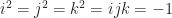
The direction of the x-axis is often written as $\hat{i}$ , and the direction of the y-axis as $\hat{j}$ . The direction of the z-axis if needed gets written $\hat{k}$ . The circumflex there indicates two things. First is that the thing underneath it is a vector. Second is that it’s a vector one unit long. A vector might have any length, including zero. It’s convenient to make some mention when it’s a nice one unit long.

Another popular notation is to write the direction of the x-axis as the vector $\hat{e}_1$ , and the y-axis as the vector $\hat{e}_2$ , and so on. This method offers several advantages. One is that we can talk about the vector $\hat{e}_j$ , that is, some particular direction without pinning down just which one. That’s the equivalent of writing “x” or “y” for a number we don’t want to commit ourselves to just yet. Another is that we can talk about axes going off in two, or three, or four, or more directions without having to pin down how many there are. And then we don’t have to think of what to call them. x- and y- and z-axes make sense. w-axis sounds a little odd but some might accept it. v-axis? u-axis? Nobody wants that, trust me.

Sometimes people start the numbering from $\hat{e}_0$ so that the y-axis is the direction $\hat{e}_1$ . Usually it’s either clear from context or else it doesn’t matter.

A Summer 2015 Mathematics A To Z: n-tuple

N-tuple.

We use numbers to represent things we want to think about. Sometimes the numbers represent real-world things: the area of our backyard, the number of pets we have, the time until we have to go back to work. Sometimes the numbers mean something more abstract: an index of all the stuff we’re tracking, or how its importance compares to other things we worry about.

Often we’ll want to group together several numbers. Each of these numbers may measure a different kind of thing, but we want to keep straight what kind of thing it is. For example, we might want to keep track of how many people are in each house on the block. The houses have an obvious index number — the street number — and the number of people in each house is just what it says. So instead of just keeping track of, say, “32” and “34” and “36”, and “3” and “2” and “3”, we would keep track of pairs: “32, 3”, and “34, 2”, and “36, 3”. These are called ordered pairs.

They’re not called ordered because the numbers are in order. They’re called ordered because the order in which the numbers are recorded contains information about what the numbers mean. In this case, the first number is the street address, and the second number is the count of people in the house, and woe to our data set if we get that mixed up.

And there’s no reason the ordering has to stop at pairs of numbers. You can have ordered triplets of numbers — (32, 3, 2), say, giving the house number, the number of people in the house, and the number of bathrooms. Or you can have ordered quadruplets — (32, 3, 2, 6), say, house number, number of people, bathroom count, room count. And so on.

An n-tuple is an ordered set of some collection of numbers. How many? We don’t care, or we don’t care to say right now. There are two popular ways to pronounce it. One is to say it the way you say “multiple” only with the first syllable changed to “enn”. Others say it about the same, but with a long u vowel, so, “enn-too-pull”. I believe everyone worries that everyone else says it the other way and that they sound like they’re the weird ones.

You might care to specify what your n is for your n-tuple. In that case you can plug in a value for that n right in the symbol: a 3-tuple is an ordered triplet. A 4-tuple is that ordered quadruplet. A 26-tuple seems like rather a lot but I’ll trust that you know what you’re trying to study. A 1-tuple is just a number. We might use that if we’re trying to make our notation consistent with something else in the discussion.

If you’re familiar with vectors you might ask: so, an n-tuple is just a vector? It’s not quite. A vector is an n-tuple, but in the same way a square is a rectangle. It has to meet some extra requirements. To be a vector we have to be able to add corresponding numbers together and get something meaningful out of it. The ordered pair (32, 3) representing “32 blocks north and 3 blocks east” can be a vector. (32, 3) plus (34, 2) can give us us (66, 5). This makes sense because we can say, “32 blocks north, 3 blocks east, 34 more blocks north, 2 more blocks east gives us 66 blocks north, 5 blocks east.” At least it makes sense if we don’t run out of city. But to add together (32, 3) plus (34, 2) meaning “house number 32 with 3 people plus house number 34 with 2 people gives us house number 66 with 5 people”? That’s not good, whatever town you’re in.

I think the commonest use of n-tuples is to talk about vectors, though. Vectors are such useful things.

Reading the Comics, March 10, 2015: Shapes Of Things Edition

If there’s a theme running through today’s collection of mathematics-themed comic strips it’s shapes: I have good reason to talk about a way of viewing circles and spheres and even squares and boxes; and then both Euclid and men’s ties get some attention.

Eric the Circle (March 5), this one by “regina342”, does a bit of shape-name-calling. I trust that it’s not controversial that a rectangle is also a parallelogram, but people might be a bit put off by describing a circle as a sphere, what with circles being two-dimensional figures and spheres three-dimensional ones. For ordinary purposes of geometry that’s a fair enough distinction. Let me now make this complicated.

Continue reading “Reading the Comics, March 10, 2015: Shapes Of Things Edition”

Combining Matrices And Model Universes

I would like to resume talking about matrices and really old universes and the way nucleosynthesis in these model universes causes atoms to keep settling down to peculiar but unchanging distribution.

I’d already described how a matrix offers a nice way to organize elements, and in ways that encode information about the context of the elements by where they’re placed. That’s useful and saves some writing, certainly, although by itself it’s not that interesting. Matrices start to get really powerful when, first, the elements being stored are things on which you can do something like arithmetic with pairs of them. Here I mostly just mean that you can add together two elements, or multiply them, and get back something meaningful.

This typically means that the matrix is made up of a grid of numbers, although that isn’t actually required, just, really common if we’re trying to do mathematics.

Then you get the ability to add together and multiply together the matrices themselves, turning pairs of matrices into some new matrix, and building something that works a lot like arithmetic on these matrices.

Adding one matrix to another is done in almost the obvious way: add the element in the first row, first column of the first matrix to the element in the first row, first column of the second matrix; that’s the first row, first column of your new matrix. Then add the element in the first row, second column of the first matrix to the element in the first row, second column of the second matrix; that’s the first row, second column of the new matrix. Add the element in the second row, first column of the first matrix to the element in the second row, first column of the second matrix, and put that in the second row, first column of the new matrix. And so on.

This means you can only add together two matrices that are the same size — the same number of rows and of columns — but that doesn’t seem unreasonable.

You can also do something called scalar multiplication of a matrix, in which you multiply every element in the matrix by the same number. A scalar is just a number that isn’t part of a matrix. This multiplication is useful, not least because it lets us talk about how to subtract one matrix from another: to find the difference of the first matrix and the second, scalar-multiply the second matrix by -1, and then add the first to that product. But you can do scalar multiplication by any number, by two or minus pi or by zero if you feel like it.

I should say something about notation. When we want to write out these kinds of operations efficiently, of course, we turn to symbols to represent the matrices. We can, in principle, use any symbols, but by convention a matrix usually gets represented with a capital letter, A or B or M or P or the like. So to add matrix A to matrix B, with the result being matrix C, we can write out the equation “A + B = C”, which is about as simple as we could hope to see. Scalars are normally written in lowercase letters, often Greek letters, if we don’t know what the number is, so that the scalar multiplication of the number r and the matrix A would be the product “rA”, and we could write the difference between matrix A and matrix B as “A + (-1)B” or “A – B”.

Matrix multiplication, now, that is done by a process that sounds like doubletalk, and it takes a while of practice to do it right. But there are good reasons for doing it that way and we’ll get to one of those reasons by the end of this essay.

To multiply matrix A and matrix B together, we do multiply various pairs of elements from both matrix A and matrix B. The surprising thing is that we also add together sets of these products, per this rule.

Take the element in the first row, first column of A, and multiply it by the element in the first row, first column of B. Add to that the product of the element in the first row, second column of A and the second row, first column of B. Add to that total the product of the element in the first row, third column of A and the third row, second column of B, and so on. When you’ve run out of columns of A and rows of B, this total is the first row, first column of the product of the matrices A and B.

Plenty of work. But we have more to do. Take the product of the element in the first row, first column of A and the element in the first row, second column of B. Add to that the product of the element in the first row, second column of A and the element in the second row, second column of B. Add to that the product of the element in the first row, third column of A and the element in the third row, second column of B. And keep adding those up until you’re out of columns of A and rows of B. This total is the first row, second column of the product of matrices A and B.

This does mean that you can multiply matrices of different sizes, provided the first one has as many columns as the second has rows. And the product may be a completely different size from the first or second matrices. It also means it might be possible to multiply matrices in one order but not the other: if matrix A has four rows and three columns, and matrix B has three rows and two columns, then you can multiply A by B, but not B by A.

My recollection on learning this process was that this was crazy, and the workload ridiculous, and I imagine people who get this in Algebra II, and don’t go on to using mathematics later on, remember the process as nothing more than an unpleasant blur of doing a lot of multiplying and addition for some reason or other.

So here is one of the reasons why we do it this way. Let me define two matrices:

$A = \left(\begin{tabular}{c c c} 3/4 & 0 & 2/5 \\ 1/4 & 3/5 & 2/5 \\ 0 & 2/5 & 1/5 \end{tabular}\right)$

$B = \left(\begin{tabular}{c} 100 \\ 0 \\ 0 \end{tabular}\right)$

Then matrix A times B is

$AB = \left(\begin{tabular}{c} 3/4 * 100 + 0 * 0 + 2/5 * 0 \\ 1/4 * 100 + 3/5 * 0 + 2/5 * 0 \\ 0 * 100 + 2/5 * 0 + 1/5 * 0 \end{tabular}\right) = \left(\begin{tabular}{c} 75 \\ 25 \\ 0 \end{tabular}\right)$

You’ve seen those numbers before, of course: the matrix A contains the probabilities I put in my first model universe to describe the chances that over the course of a billion years a hydrogen atom would stay hydrogen, or become iron, or become uranium, and so on. The matrix B contains the original distribution of atoms in the toy universe, 100 percent hydrogen and nothing anything else. And the product of A and B was exactly the distribution after that first billion years: 75 percent hydrogen, 25 percent iron, nothing uranium.

If we multiply the matrix A by that product again — well, you should expect we’re going to get the distribution of elements after two billion years, that is, 56.25 percent hydrogen, 33.75 percent iron, 10 percent uranium, but let me write it out anyway to show:

$\left(\begin{tabular}{c c c} 3/4 & 0 & 2/5 \\ 1/4 & 3/5 & 2/5 \\ 0 & 2/5 & 1/5 \end{tabular}\right)\left(\begin{tabular}{c} 75 \\ 25 \\ 0 \end{tabular}\right) = \left(\begin{tabular}{c} 3/4 * 75 + 0 * 25 + 2/5 * 0 \\ 1/4 * 75 + 3/5 * 25 + 2/5 * 0 \\ 0 * 75 + 2/5 * 25 + 1/5 * 0 \end{tabular}\right) = \left(\begin{tabular}{c} 56.25 \\ 33.75 \\ 10 \end{tabular}\right)$

And if you don’t know just what would happen if we multipled A by that product, you aren’t paying attention.

This also gives a reason why matrix multiplication is defined this way. The operation captures neatly the operation of making a new thing — in the toy universe case, hydrogen or iron or uranium — out of some combination of fractions of an old thing — again, the former distribution of hydrogen and iron and uranium.

Or here’s another reason. Since this matrix A has three rows and three columns, you can multiply it by itself and get a matrix of three rows and three columns out of it. That matrix — which we can write as A² — then describes how two billion years of nucleosynthesis would change the distribution of elements in the toy universe. A times A times A would give three billion years of nucleosynthesis; A¹⁰ ten billion years. The actual calculating of the numbers in these matrices may be tedious, but it describes a complicated operation very efficiently, which we always want to do.

I should mention another bit of notation. We usually use capital letters to represent matrices; but, a matrix that’s just got one column is also called a vector. That’s often written with a lowercase letter, with a little arrow above the letter, as in $\vec{x}$ , or in bold typeface, as in x. (The arrows are easier to put in writing, the bold easier when you were typing on typewriters.) But if you’re doing a lot of writing this out, and know that (say) x isn’t being used for anything but vectors, then even that arrow or boldface will be forgotten. Then we’d write the product of matrix A and vector x as just Ax. (There are also cases where you put a little caret over the letter; that’s to denote that it’s a vector that’s one unit of length long.)

When you start writing vectors without an arrow or boldface you start to run the risk of confusing what symbols mean scalars and what ones mean vectors. That’s one of the reasons that Greek letters are popular for scalars. It’s also common to put scalars to the left and vectors to the right. So if one saw “rMx”, it would be expected that r is a scalar, M a matrix, and x a vector, and if they’re not then this should be explained in text nearby, preferably before the equations. (And of course if it’s work you’re doing, you should know going in what you mean the letters to represent.)

Orthonormal.

Kindly share this:

Velocity.

Kindly share this:

J Willard Gibbs.

Kindly share this:

Norm.

Kindly share this:

Kindly share this:

Kindly share this:

Hat.

Kindly share this:

Kindly share this:

Vector.

Kindly share this:

Quaternion.

Kindly share this:

Orthonormal.

Kindly share this:

Energy.

Kindly share this:

Rn

Kindly share this:

Kindly share this:

y-axis.

Kindly share this:

N-tuple.

Kindly share this:

Kindly share this:

Kindly share this:

Rⁿ