And now, finally, the close of the All 2020 Mathematics A-to-Z. You may see this as coming in after the close of 2020. I say, well, I’ve done that before. Things that come close to the end of the year are prone to that.
The first important lesson was that I need to read exactly what topics I’ve written about before going ahead with a new week’s topic. I am not sorry, really, to have written about Tiling a second time. I’d rather it have been more than two years after the previous time. But I can make a little something out of that, too. I enjoy the second essay more. I don’t think that’s only because I like my most recent writing more. In the second version I looked at one of those fussy little specific questions. Particularly, what were the 20,426 tiles which Robert Berger found could create an aperiodic tiling? Tracking that down brought me to some fun new connections. And it let me write in a less foggy way. It’s always tempting to write the most generally true thing possible. But details and example cases are easier to understand. It’s surprising that no one in the history of knowledge has observed this difference before I did.
The second lesson was about work during a crisis. 2020 was the most stressful year of my life, a fact I hope remains true. I am aware that ritual, doing regular routine things, helps with stress. So a regular schedule of composing an essay on a mathematical topic was probably a good thing for me. Committing to the essay meant I had specific, attainable goals on clear, predictable deadlines. The catch is that I never got on top of the A-to-Z the way I hoped. My ideal for these is to have the essay written a week ahead of publication. Enough that I can sleep on it many times and amend it as needed. I never got close to this. I was running up close to deadline every week. If I were better managing all this I’d have gotten all November’s essays written before the election, and I didn’t, and that’s why I had to slip a week. I have always been a Sabbath-is-made-for-man sort, so don’t feel bad for slipping the week. But I would have liked to never had had a week when I was copy-editing a half-hour before publication.
It does all imply that I need to do what I resolve every year. Select topics sooner. Start research and drafts sooner. Let myself slip a deadline when that’s needed. But there is also the observation that apparently I can’t cut down the time I spend writing. The first several years of this, believe it or not, I wrote three essays a week for eight intense weeks. These would be six to eight hundred words each. Then I slacked off, doing two a week; these of course grew to a thousand, maybe 1200 words each. For 2020? One essay a week and more than one topped 2500 words. Yes, the traditional joke is that you write a lot because you don’t have the time to write briefly. But writing a lot takes time too.
The third lesson is about biographies. I wrote more biographical sketches for 2020’s than for any previous A-to-Z. Six, if I’m not miscounting, and that without counting historical pieces like Hilbert’s Problems or statistics. These biographies had enlightening minor discoveries. Here I mean learning that Fibonacci seems to have been much less important than I’d imagined. They’re great fun to write, and a different set of challenges from describing what a cohomology might be.
They’re challenging. In the pandemic particularly, as I can’t rely on the university library for a quick biography to read. Or to check journals of mathematical history, although I haven’t resorted to such actual information yet. But I’m also aware that I am not a historian or a real biographer. I have to balance drawing conclusions I can feel confident are not wrong with making declarations that are interesting to read. Still, I enjoy a focus on the culture of mathematics, and how mathematics interacts with the broader culture. It’s a piece mathematicians tend not to acknowledge; our field’s reputation for objective truth is a compelling romantic legend.
I do plan to write an A-to-Z for 2021. I suspect I’ll do it as this year, one per week. I don’t know when I’ll start, although it should be earlier than June. I’ll want to give myself more possible slip dates without running off the year. I will not be writing about tiling again. I do realize that, since I have seven A-to-Z sequences of 26 essays each, I could in principle fill half a year with writing by reblogging each, one a day. I’m not sure the point of such an exercise, but it would at least fill the content hole.
There is a side of me that would like to have a blogging gimmick that doesn’t commit me to 26 essays. I’ve tried a couple; they haven’t ever caught like this has. Maybe I could do something small and focused, like, ten terms from complex analysis. I’m open to suggestions.
When will I resume covering mathematical themes in comic strips? I don’t know; it’s the obvious thing to do while I wait for the A-to-Z cycle to start anew. It’s got some of the A-to-Z thrill, of writing about topics someone else chose. But I need some time to relax and play and I don’t know when I’ll be back to regular work.
I am happy, as ever, to complete an A-to-Z. Also to take some time to recover after the project. I had thought that spreading things out to 26 weeks would make them less stressful, and instead, I just wrote even longer pieces, in compensation. I’ll try to have other good observations in an essay next week.
For now, though, a piece that I will find useful for years to come: a roster of what essays I wrote this year. In future years, I may even check them before writing a third piece about tiling.
Jacob Siehler had several suggestions for this last of the A-to-Z essays for 2020. Zorn’s Lemma was an obvious choice. It’s got an important place in set theory, it’s got some neat and weird implications. It’s got a great name. The zero divisor is one of those technical things mathematics majors have deal with. It never gets any pop-mathematics attention. I picked the less-travelled road and found a delightful scenic spot.
3 times 4 is 12. That’s a clear, unambiguous, and easily-agreed-upon arithmetic statement. The thing to wonder is what kind of mathematics it takes to mess that up. The answer is algebra. Not the high school kind, with x’s and quadratic formulas and all. The college kind, with group theory and rings.
A ring is a mathematical construct that lets you do a bit of arithmetic. Something that looks like arithmetic, anyway. It has a set of elements. (An element is just a thing in a set. We say “element” because it feels weird to call it “thing” all the time.) The ring has an addition operation. The ring has a multiplication operation. Addition has an identity element, something you can add to any element without changing the original element. We can call that ‘0’. The integers, or to use the lingo , are a ring (among other things).
Among the rings you learn, after the integers, is the integers modulo … something. This can be modulo any counting number. The integers modulo 10, for example, we write as for short. There are different ways to think of what this means. The one convenient for this essay is that it’s the integers 0, 1, 2, up through 9. And that the result of any calculation is “how much more than a whole multiple of 10 this calculation would otherwise be”. So then 3 times 4 is now 2. 3 times 5 is 5; 3 times 6 is 8. 3 times 7 is 1, and doesn’t that seem peculiar? That’s part of how modulo arithmetic warns us that groups and rings can be quite strange things.
We can do modulo arithmetic with any of the counting numbers. Look, for example, at instead. In the integers modulo 5, 3 times 4 is … 2. This doesn’t seem to get us anything new. How about ? In this, 3 times 4 is 4. That’s interesting. It doesn’t make 3 the multiplicative identity for this ring. 3 times 3 is 1, for example. But you’d never see something like that for regular arithmetic.
How about ? Now we have 3 times 4 equalling 0. And that’s a dramatic break from how regular numbers work. One thing we know about regular numbers is that if a times b is 0, then either a is 0, or b is zero, or they’re both 0. We rely on this so much in high school algebra. It’s what lets us pick out roots of polynomials. Now? Now we can’t count on that.
When this does happen, when one thing times another equals zero, we have “zero divisors”. These are anything in your ring that can multiply by something else to give 0. Is zero, the additive identity, always a zero divisor? … That depends on what the textbook you first learned algebra from said. To avoid ambiguity, you can write a “nonzero zero divisor”. This clarifies your intentions and slows down your copy editing every time you read “nonzero zero”. Or call it a “nontrivial zero divisor” or “proper zero divisor” instead. My preference is to accept 0 as always being a zero divisor. We can disagree on this. What of zero divisors other than zero?
Your ring might or might not have them. It depends on the ring. The ring of integers , for example, doesn’t have any zero divisors except for 0. The ring of integers modulo 12 , though? Anything that isn’t relatively prime to 12 is a zero divisor. So, 2, 3, 6, 8, 9, and 10 are zero divisors here. The ring of integers modulo 13 ? That doesn’t have any zero divisors, other than zero itself. In fact any ring of integers modulo a prime number, , lacks zero divisors besides 0.
Focusing too much on integers modulo something makes zero divisors sound like some curious shadow of prime numbers. There are some similarities. Whether a number is prime depends on your multiplication rule and what set of things it’s in. Being a zero divisor in one ring doesn’t directly relate to whether something’s a zero divisor in any other. Knowing what the zero divisors are tells you something about the structure of the ring.
It’s hard to resist focusing on integers-modulo-something when learning rings. They work very much like regular arithmetic does. Even the strange thing about them, that every result is from a finite set of digits, isn’t too alien. We do something quite like it when we observe that three hours after 10:00 is 1:00. But many sets of elements can create rings. Square matrixes are the obvious extension. Matrixes are grids of elements, each of which … well, they’re most often going to be numbers. Maybe integers, or real numbers, or complex numbers. They can be more abstract things, like rotations or whatnot, but they’re hard to typeset. It’s easy to find zero divisors in matrixes of numbers. Imagine, like, a matrix that’s all zeroes except for one element, somewhere. There are a lot of matrices which, multiplied by that, will be a zero matrix, one with nothing but zeroes in it. Another common kind of ring is the polynomials. For these you need some constraint like the polynomial coefficients being integers-modulo-something. You can make that work.
In 1988 Istvan Beck tried to establish a link between graph theory and ring theory. We now have a usable standard definition of one. If is any ring, then is the zero-divisor graph of . (I know some of you think is the real numbers. No; that’s a bold-faced instead. Unless that’s too much bother to typeset.) You make the graph by putting in a vertex for the elements in . You connect two vertices a and b if the product of the corresponding elements is zero. That is, if they’re zero divisors for one other. (In Beck’s original form, this included all the elements. In modern use, we don’t bother including the elements that are not zero divisors.)
Drawing this graph makes tools from graph theory available to study rings. We can measure things like the distance between elements, or what paths from one vertex to another exist. What cycles — paths that start and end at the same vertex — exist, and how large they are. Whether the graphs are bipartite. A bipartite graph is one where you can divide the vertices into two sets, and every edge connects one thing in the first set with one thing in the second. What the chromatic number — the minimum number of colors it takes to make sure no two adjacent vertices have the same color — is. What shape does the graph have?
It’s easy to think that zero divisors are just a thing which emerges from a ring. The graph theory connection tells us otherwise. You can make a potential zero divisor graph and ask whether any ring could fit that. And, from that, what we can know about a ring from its zero divisors. Mathematicians are drawn as if by an occult hand to things that let you answer questions about a thing from its “shape”.
And this lets me complete a cycle in this year’s A-to-Z, to my delight. There is an important question in topology which group theory could answer. It’s a generalization of the zero-divisors conjecture, a hypothesis about what fits in a ring based on certain types of groups. This hypothesis — actually, these hypotheses. There are a bunch of similar questions about invariants called the L2-Betti numbers can be. These we call the Atiyah Conjecture. This because of work Michael Atiyah did in the cohomology of manifolds starting in the 1970s. It’s work, I admit, I don’t understand well enough to summarize, and hope you’ll forgive me for that. I’m still amazed that one can get to cutting-edge mathematics research this. It seems, at its introduction, to be only a subversion of how we find x for which .
Nobody had particular suggestions for the letter ‘Y’ this time around. It’s a tough letter to find mathematical terms for. It doesn’t even lend itself to typography or wordplay the way ‘X’ does. So I chose to do one more biographical piece before the series concludes. There were twists along the way in writing.
Before I get there, I have a word for a longtime friend, Porsupah Ree. Among her hobbies is watching, and photographing, the wild rabbits. A couple years back she got a great photograph. It’s one that you may have seen going around social media with a caption about how “everybody was bun fu fighting”. She’s put it up on Redbubble, so you can get the photograph as a print or a coffee mug or a pillow, or many other things. And you can support her hobbies of rabbit photography and eating.
Several problems beset me in writing about this significant 13th-century Chinese mathematician. One is my ignorance of the Chinese mathematical tradition. I have little to guide me in choosing what tertiary sources to trust. Another is that the tertiary sources know little about him. The Complete Dictionary of Scientific Biography gives a dire verdict. “Nothing is known about the life of Yang Hui, except that he produced mathematical writings”. MacTutor’s biography gives his lifespan as from circa 1238 to circa 1298, on what basis I do not know. He seems to have been born in what’s now Hangzhou, near Shanghai. He seems to have worked as a civil servant. This is what I would have imagined; most scholars then were. It’s the sort of job that gives one time to write mathematics. Also he seems not to have been a prominent civil servant; he’s apparently not listed in any dynastic records. After that, we need to speculate.
E F Robertson, writing the MacTutor biography, speculates that Yang Hui was a teacher. That he was writing to explain mathematics in interesting and helpful ways. I’m not qualified to judge Robertson’s conclusions. And Robertson notes that’s not inconsistent with Yang being a civil servant. Robertson’s argument is based on Yang’s surviving writings, and what they say about the demonstrated problems. There is, for example, 1274’s Cheng Chu Tong Bian Ben Mo. Robertson translates that title as Alpha and omega of variations on multiplication and division. I try to work out my unease at having something translated from Chinese as “Alpha and Omega”. That is my issue. Relevant here is that a syllabus prefaces the first chapter. It provides a schedule and series of topics, as well as a rationale for why this plan.
Was Yang Hui a discoverer of significant new mathematics? Or did he “merely” present what was already known in a useful way? This is not to dismiss him; we have the same questions about Euclid. He is held up as among the great Chinese mathematicians of the 13th century, a particularly fruitful time and place for mathematics. How much greatness to assign to original work and how much to good exposition is unanswerable with what we know now.
Consider for example the thing I’ve featured before, Yang Hui’s Triangle. It’s the arrangement of numbers known in the west as Pascal’s Triangle. Yang provides the earliest extant description of the triangle and how to form it and use it. This in the 1261 Xiangjie jiuzhang suanfa (Detailed analysis of the mathematical rules in the Nine Chapters and their reclassifications). But in it, Yang Hui says he learned the triangle from a treatise by Jia Xian, Huangdi Jiuzhang Suanjing Xicao (The Yellow Emperor’s detailed solutions to the Nine Chapters on the Mathematical Art). Jia Xian lived in the 11th century; he’s known to have written two books, both lost. Yang Hui’s commentary gives us a fair idea what Jia Xian wrote about. But we’re limited in judging what was Jia Xian’s idea and what was Yang Hui’s inference or what.
The Nine Chapters referred to is Jiuzhang suanshu. An English title is Nine Chapters on the Mathematical Art. The book is a 246-problem handbook of mathematics that dates back to antiquity. It’s impossible to say when the Nine Chapters was first written. Liu Hui, who wrote a commentary on the Nine Chapters in 263 CE, thought it predated the Qin ruler Shih Huant Ti’s 213 BCE destruction of all books. But the book — and the many commentaries on the book — served as a centerpiece for Chinese mathematics for a long while. Jia Xian’s and Yang Hui’s work was part of this tradition.
Yang Hui’s Detailed Analysis covers the Nine Chapters. It goes on for three chapters, more about geometry and fundamentals of mathematics. Even how to classify the problems. He had further works. In 1275 Yang published Practical mathematical rules for surveying and Continuation of ancient mathematical methods for elucidating strange properties of numbers. (I’m not confident in my ability to give the Chinese titles for these.) The first title particularly echoes how in the Western tradition geometry was born of practical concerns.
The breadth of topics covers, it seems to me, a decent modern (American) high school mathematics education. The triangle, and the binomial expansions it gives us, fit that. Yang writes about more efficient ways to multiply on the abacus. He writes about finding simultaneous solutions to sets of equations. And through a technique that amounts to finding the matrix of coefficients for the equations, and its determinant. He writes about finding the roots for cubic and quartic equations. The technique is commonly known in the west as Horner’s Method, a technique of calculating divided differences. We see the calculating of areas and volumes for regular shapes.
And sequences. He found the sum of the squares of natural numbers followed a rule:
This by a method of “piling up squares”, described some here by the Mathematical Association of America. (Me, I spent 40 minutes that could have gone into this essay convincing myself the formula was right. I couldn’t make myself believe the part and had to work it out a couple different ways.)
And then there’s magic squares, and magic circles. He seems to have found them, as professional mathematicians today would, good ways to interest people in calculation. Not magic; he called them something like number diagrams. But he gives magic squares from three-by-three all the way to ten-by-ten. We don’t know of earlier examples of Chinese mathematicians writing about the larger magic squares. But Yang Hui doesn’t claim to be presenting new work. He also gives magic circles. The simplest is a web of seven intersecting circles, each with four numbers along the circle and one at its center. The sum of the center and the circumference numbers are 65 for all seven circles. Is this significant? No; merely fun.
Grant this breadth of work. Is he significant? I learned this year that familiar names might have been obscure until quite recently. The record is once again ambiguous. Other mathematicians wrote about Yang Hui’s work in the early 1300s. Yang Hui’s works were printed in China in 1378, says the Complete Dictionary of Scientific Biography, and reprinted in Korea in 1433. They’re listed in a 1441 catalogue of the Ming Imperial Library. Seki Takakazu, a towering figure in 17th century Japanese mathematics, copied the Korean text by hand. Yet Yang Hui’s work seems to have been lost by the 18th century. Reconstructions, from commentaries and encyclopedias, started in the 19th century. But we don’t have everything we know he wrote. We don’t even have a complete text of Detailed Analysis. This is not to say he wasn’t influential. All I could say is there seems to have been a time his influence was indirect.
When developing general relativity, Albert Einstein created a convention. He’s not unique in that. All mathematicians create conventions. They use shorthand for an idea that’s complicated or common. Relatively unique is that other people adopted his convention, because it expressed an idea compactly. This was in working with tensors, which look somewhat like matrixes and have a lot of indexes. In the equations of general relativity you need to take sums over many combinations of values of these indexes. What indexes there are are the same in most every problem. The possible values of the indexes is constant, problem to problem, too.
So Einstein saved himself writing, and his publishers from typesetting, a lot of redundant writing. This by writing out the conditions which implied “take the sums over these indexes on this range”. This is good for people doing general relativity, and certain kinds of geometry. It’s a problem only when an expression escapes its context. When it’s shown to a student or someone who doesn’t know this is a differential-geometry problem. Then the problem becomes confusing, and they can’t work on it.
This is not to fault the Einstein Summation Convention. It puts common necessary scaffolding out of the way and highlighting the interesting unique parts of a problem. Most conventions aim for that. We have the hazard, though, that we may not notice something breaking the convention.
And this is how we create extraneous solutions. And, as a bonus, to have missing solutions. We encounter them with the start of (high school) algebra, when we get used to manipulating equations. When we solve an equation what we always want is something clear, like
But it never starts that way. It always starts with something like
or worse. We learn how to handle this. We know that we can do six things that do not alter the truth of an equation. We can regroup terms in the equation. We can add the same number to both sides of the equation. We can multiply both sides of the equation by some number besides zero. We can add zero to one side of the equation. We can multiply one side of the equation by 1. We can replace one quantity with another that has the same value. That doesn’t sound like a lot. It covers more than it seems. Multiplying by 1, for example, is the same as multiplying by . If x isn’t zero, then we can multiply both sides of the equation by that x. And x can’t be zero, or else would not be 1.
So with my example there, start off by multiplying the right side by 1, in the guise . Then multiply both sides by that same non-zero x. At this point the right-hand side simplifies to being 6. Add a -6 to both sides. And then with a lot of shuffling around you work out that the equation is the same as
And that can only be true when x equals 2.
It should be easy to catch spurious solutions creeping in. They must result from breaking a rule. The obvious problem is multiplying — or dividing — by zero. We expect those to be trouble. Wikipedia has a fine example:
The obvious step is to multiply this whole mess by , which turns our work into a linear equation. Very soon we find the solution must be . Which would make at least two of the denominators in the original equation zero. We know not to want that.
The problems can be subtler, though. Consider:
That’s not hard to solve. Multiply both sides by . Although, before working out substitute that with something equal to it. We know one thing is equal to it, . Then we have
It’s a quadratic equation. A little bit of work shows the roots are 9 and 16. One of those answers is correct and the other spurious. At no point did we divide anything, by zero or anything else.
So what is happening and what is the necessary rhetorical link to the Einstein Summation Convention?
There are many ways to look at equations. One that’s common is to look at them as functions. This is so common that we’ll elide between an equation and a function representation. This confuses the prealgebra student who wants to know why sometimes we look at
and sometimes we look at
and sometimes at
The advantage of looking at the function which shadows any equation is we have different tools for studying functions. Sometimes that makes solving the equation easier. In this form, we’re looking for what in the domain matches with something particular in the range.
And now we’ve reached the convention. When we write down something lke we’re implicitly defining a function. A function has three pieces. It has a set called the domain, from which we draw the independent variable. It has a set called the range. It has a rule matching elements in the domain to an element in the range. We’ve only given the rule. What are the domain and what’s the range for ?
And here are the conventions. If we haven’t said otherwise, the domain and range are usually either the real numbers or the complex numbers. If we used x or y or t as the independent variable, we mean the real numbers. If we used z as the independent variable, and haven’t already put x and y in, we mean the complex numbers. Sometimes we call in s or w or another letter; never mind that. The range can be the whole set of real or complex numbers. It does us no harm to have too large a range.
The domain, though. We do insist that everything in the domain match to something in the range. And, like, ? That can’t mean anything if x equals 2.
So we take an implicit definition of the domain: it’s all the real numbers for which the function’s rule is meaningful. So, would have a domain “real numbers other than 2”. would have a domain “real numbers other than 2 and -2”.
We create extraneous solutions — or we lose some — when our convention changes the domain. An extraneous solution is one that existed outside the original problem’s domain. A missing solution is one that existed in an excised part of the domain. To go from to by dividing out x is to cut out of the space of possible solutions.
A complaint you might raise. What is the domain for ? Rewrite that as a function. would seem to have a domain “x greater than or equal to 0”. The extraneous solution is , a number which rumor has it is greater than or equal to 0. What happened?
We have to take that equation-handling more slowly. We had started out with
The domain has to be “x is greater than or equal to 0” here. All right. The next step was multiplying both sides by the same quantity, . So:
The domain is still “x is greater than or equal to 0”. The next step, though, was a substitution. I wanted to replace the on the right with . We know, from the original equation, that those are equal. At least, they’re equal wherever the original equation is true. What happens when , though?
We start to see the catch. 9 – 12 is -3. And while it’s true that -3 squared will be 9, it’s false that -3 is the square root of 9. The equation can only be true, for real numbers, if is nonnegative. We can make this rigorous with two supplementary functions. Let me call and .
has an implicit domain of “x greater than or equal to 0”. What’s the domain of ? If , like we said it does, then they have to agree for every x in either’s domain. So can’t have in its domain any x for which isn’t defined. So the domain of has to be “x for which x – 12 is greater than or equal to 0”. And that’s “x greater than or equal to 12”.
So the domain for the original equation is “x greater than or equal to 12”. When we keep that domain in mind, the extraneous nature of is clear, and we avoid trouble.
Not all extraneous solutions come from algebraic manipulations. Sometimes there are constraints on the problem, rather than the numbers, that make a solution absurd. There is a betting strategy called the martingale. This amounts to doubling the bet every time one loses. This makes the first win balance out all the losses leading to it. This solution fails because the player has a finite wallet, and after a few losses any player hasn’t got the money to continue.
Or consider a case that may be legend. It concerns the Apollo Guidance Computer. It was designed to take the Lunar Module to a spot at zero altitude above the moon’s surface, with zero velocity. The story is that in early test runs, the computer would not avoid trajectories that dropped to a negative altitude along the way to the surface. One imagines the scene after the first Apollo subway trip. (I have not found a date when such a test run was done, or corrections to the code ordered. If someone knows, I’d appreciate learning specifics.)
The convention, that we trust the domain is “everything which makes sense”, is not to blame here. It’s normally a good convention. Explicitly noting the domain at every step is tedious and, most of the time, unenlightening. It belongs in the background. We also must check our possible solutions, and that they represent things that make sense. We can try to concentrate our thinking on the obvious interesting parts, but must spend some time on the rest also.
Today’s is another topic suggested by Mr Wu, author of the Singapore Maths Tuition blog. The Wronskian is named for Józef Maria Hoëne-Wroński, a Polish mathematician, born in 1778. He served in General Tadeusz Kosciuszko’s army in the 1794 Kosciuszko Uprising. After being captured and forced to serve in the Russian army, he moved to France. He kicked around Western Europe and its mathematical and scientific circles. I’d like to say this was all creative and insightful, but, well. Wikipedia describes him trying to build a perpetual motion machine. Trying to square the circle (also impossible). Building a machine to predict the future. The St Andrews mathematical biography notes his writing a summary of “the general solution of the fifth degree [polynomial] equation”. This doesn’t exist.
Both sources, though, admit that for all that he got wrong, there were flashes of insight and brilliance in his work. The St Andrews biography particularly notes that Wronski’s tables of logarithms were well-designed. This is a hard thing to feel impressed by. But it’s hard to balance information so that it’s compact yet useful. He wrote about the Wronskian in 1812; it wouldn’t be named for him until 1882. This was 29 years after his death, but it does seem likely he’d have enjoyed having a familiar thing named for him. I suspect he wouldn’t enjoy my next paragraph, but would enjoy the fight with me about it.
The Wronskian is a thing put into Introduction to Ordinary Differential Equations courses because students must suffer in atonement for their sins. Those who fail to reform enough must go on to the Hessian, in Partial Differential Equations.
To be more precise, the Wronskian is the determinant of a matrix. The determinant you find by adding and subtracting products of the elements in a matrix together. It’s not hard, but it is tedious, and gets more tedious pretty fast as the matrix gets bigger. (In Big-O notation, it’s the order of the cube of the matrix size. This is rough, for things humans do, although not bad as algorithms go.) The matrix here is made up of a bunch of functions and their derivatives. The functions need to be ones of a single variable. The derivatives, you need first, second, third, and so on, up to one less than the number of functions you have.
If you have two functions, and , you need their first derivatives, and . If you have three functions, , , and , you need first derivatives, , , and , as well as second derivatives, , , and . If you have functions and here I’ll call them , you need derivatives, and so on through . You see right away this is a fun and exciting thing to calculate. Also why in intro to differential equations you only work this out with two or three functions. Maybe four functions if the class has been really naughty.
Go through your functions and your derivatives and make a big square matrix. And then you go through calculating the derivative. This involves a lot of multiplying strings of these derivatives together. It’s a lot of work. But at least doing all this work gets you older.
So one will ask why do all this? Why fit it into every Intro to Ordinary Differential Equations textbook and why slip it in to classes that have enough stuff going on?
One answer is that if the Wronskian is not zero for some values of the independent variable, then the functions that went into it are linearly independent. Mathematicians learn to like sets of linearly independent functions. We can treat functions like directions in space. Linear independence assures us none of these functions are redundant, pointing a way we already can describe. (Real people see nothing wrong in having north, east, and northeast as directions. But mathematicians would like as few directions in our set as possible.) The Wronskian being zero for every value of the independent variable seems like it should tell us the functions are linearly dependent. It doesn’t, not without some more constraints on the functions.
This is fine, but who cares? And, unfortunately, in Intro it’s hard to reach a strong reason to care. To this major, the emphasis on linearly independent functions felt misplaced. It’s the sort of thing we care about in linear algebra. Or some course where we talk about vector spaces. Differential equations do lead us into vector spaces. It’s hard to find a corner of analysis that doesn’t.
Every ordinary differential equation has a secret picture. This is a vector field. One axis in the field is the independent variable of the function. The other axes are the value of the function. And maybe its derivatives, depending on how many derivatives are used in the ordinary differential equation. To solve one particular differential equation is to find one path in this field. People who just use differential equations will want to find one path.
Mathematicians tend to be fine with finding one path. But they want to find what kinds of paths there can be. Are there paths which the differential equation picks out, by making paths near it stay near? Or by making paths that run away from it? And here is the value of the Wronskian. The Wronskian tells us about the divergence of this vector field. This gives us insight to how these paths behave. It’s in the same way that knowing where high- and low-pressure systems are describes how the weather will change. The Wronskian, by way of a thing called Liouville’s Theorem that I haven’t the strength to describe today, ties in to the Hamiltonian. And the Hamiltonian we see in almost every mechanics problem of note.
You can see where the mathematics PhD, or the physicist, would find this interesting. But what about the student, who would look at the symbols evoked by those paragraphs above with reasonable horror?
And here’s the second answer for what the Wronskian is good for. It helps us solve ordinary differential equations. Like, particular ones. An ordinary differential equation will (normally) have several linearly independent solutions. If you know all but one of those solutions, it’s possible to calculate the Wronskian and, from that, the last of the independent solutions. Since a big chunk of mathematics — particularly for science or engineering — is solving differential equations you see why this is something valuable. Allow that it’s tedious. Tedious work we can automate, or give to research assistant to do.
One then asks what kind of differential equation would have all-but-one answer findable, and yield that last one only by long efforts of hard work. So let me show you an example ordinary differential equation:
Here , , and are some functions that depend only on the independent variable, . Don’t know what they are; don’t care. The differential equation is a lot easier of and are constants, but we don’t insist on that.
This equation has a close cousin, and one that’s easier to solve than the original. Is cousin is called a homogeneous equation:
The left-hand-side, the parts with the function that we want to find, is the same. It’s the right-hand-side that’s different, that’s a constant zero. This is what makes the new equation homogenous. This homogenous equation is easier and we can expect to find two functions, and , that solve it. If and are constant this is even easy. Even if they’re not, if you can find one solution, the Wronskian lets you generate the second.
That’s nice for the homogenous equation. But if we care about the original, inhomogenous one? The Wronskian serves us there too. Imagine that the inhomogenous solution has any solution, which we’ll call . (The ‘p’ stands for ‘particular’, as in “the solution for this particular ”.) But also has to solve that inhomogenous differential equation. It seems startling but if you work it out, it’s so. (The key is the derivative of the sum of functions is the same as the sum of the derivative of functions.) also has to solve that inhomogenous differential equation. In fact, for any constants and , it has to be that is a solution.
I’ll skip the derivation; you have Wikipedia for that. The key is that knowing these homogenous solutions, and the Wronskian, and the original , will let you find the that you really want.
My reading is that this is more useful in proving things true about differential equations, rather than particularly solving them. It takes a lot of paper and I don’t blame anyone not wanting to do it. But it’s a wonder that it works, and so well.
Don’t make your instructor so mad you have to do the Wronskian for four functions.
This is easy. The velocity is the first derivative of the position. First derivative with respect to time, if you must know. That hardly needed an extra week to write.
Yes, there’s more. There is always more. Velocity is important by itself. It’s also important for guiding us into new ideas. There are many. One idea is that it’s often the first good example of vectors. Many things can be vectors, as mathematicians see them. But the ones we think of most often are “some magnitude, in some direction”.
The position of things, in space, we describe with vectors. But somehow velocity, the changes of positions, seems more significant. I suspect we often find static things below our interest. I remember as a physics major that my Intro to Mechanics instructor skipped Statics altogether. There are many important things, like bridges and roofs and roller coaster supports, that we find interesting because they don’t move. But the real Intro to Mechanics is stuff in motion. Balls rolling down inclined planes. Pendulums. Blocks on springs. Also planets. (And bridges and roofs and roller coaster supports wouldn’t work if they didn’t move a bit. It’s not much though.)
So velocity shows us vectors. Anything could, in principle, be moving in any direction, with any speed. We can imagine a thing in motion inside a room that’s in motion, its net velocity being the sum of two vectors.
And they show us derivatives. A compelling answer to “what does differentiation mean?” is “it’s the rate at which something changes”. Properly, we can take the derivative of any quantity with respect to any variable. But there are some that make sense to do, and position with respect to time is one. Anyone who’s tried to catch a ball understands the interest in knowing.
We take derivatives with respect to time so often we have shorthands for it, by putting a ‘ mark after, or a dot above, the variable. So if x is the position (and it often is), then is the velocity. If we want to emphasize we think of vectors, is the position and the velocity.
Velocity has another common shorthand. This is , or if we want to emphasize its vector nature, . Why a name besides the good enough ? It helps us avoid misplacing a ‘ mark in our work, for one. And giving velocity a separate symbol encourages us to think of the velocity as independent from the position. It’s not — not exactly — independent. But knowing that a thing is in the lawn outside tells us nothing about how it’s moving. Velocity affects position, in a process so familiar we rarely consider how there’s parts we don’t understand about it. But velocity is also somehow also free of the position at an instant.
Velocity also guides us into a first understanding of how to take derivatives. Thinking of the change in position over smaller and smaller time intervals gets us to the “instantaneous” velocity by doing only things we can imagine doing with a ruler and a stopwatch.
Velocity has a velocity. , also known as . Or, if we’re sure we won’t lose a ‘ mark, . Once we are comfortable thinking of how position changes in time we can think of other changes. Velocity’s change in time we call acceleration. This is also a vector, more abstract than position or velocity. Multiply the acceleration by the mass of the thing accelerating and we have a vector called the “force”. That, we at least feel we understand, and can work with.
Acceleration has a velocity too, a rate of change in time. It’s called the “jerk” by people telling you the change in acceleration in time is called the “jerk”. (I don’t see the term used in the wild, but admit my experience is limited.) And so on. We could, in principle, keep taking derivatives of the position and keep finding new changes. But most physics problems we find interesting use just a couple of derivatives of the position. We can label them, if we need, , where n is some big enough number like 4.
We can bundle them in interesting ways, though. Come back to that mention of treating position and velocity of something as though they were independent coordinates. It’s a useful perspective. Imagine the rules about how particles interacting with one another and with their environment. These usually have explicit roles for position and velocity. (Granting this may reflect a selection bias. But these do cover enough interesting problems to fill a career.)
So we create a new vector. It’s made of the positition and the velocity. We’d write it out as . The superscript-T there, “transposition”, lets us use the tools of matrix algebra. This vector describes a point in phase space. Phase space is the collection of all the physically possible positions and velocities for the system.
What’s the derivative, in time, of this point in phase space? Glad to say we can do this piece by piece. The derivative of a vector is the derivative of each component of a vector. So the derivative of is , or, . This acceleration itself depends on, normally, the positions and velocities. So we can describe this as for some function . You are surely impressed with this symbol-shuffling. You are less sure why this bother.
The bother is a trick of ordinary differential equations. All differential equations are about how a function-to-be-determined and its derivatives relate to one another. In ordinary differential equations, the function-to-be-determined depends on a single variable. Usually it’s called x or t. There may be many derivatives of f. This symbol-shuffling rewriting takes away those higher-order derivatives. We rewrite the equation as a vector equation of just one order. There’s some point in phase space, and we know what its velocity is. That we do because in this form many problems can be written as a matrix problem: . Or approximate our problem as a matrix problem. This lets us bring in linear algebra tools, and that’s worthwhile.
It also lets us bring in numerical tools. Numerical mathematics has developed many methods to solve the ordinary differential equation. Most of them extend to . The result is a classic mathematician’s trick. We can recast a problem as one we have better tools to solve.
It calls on a more abstract idea of what a “velocity” might be. We can explain what the thing that’s “moving” and what it’s moving through are, given time. But the instincts we develop from watching ordinary things move help us in these new territories. This is also a classic mathematician’s trick. It may seem like all mathematicians do is develop tricks to extend what they already do. I can’t say this is wrong.
I decided to let the V essay slide to Wednesday. This will make the end of the 2020 A-to-Z run a week later than I originally imagined, but that’s all right. It’ll all end in 2020 unless there’s another unexpected delay.
I have gotten several good suggestions for the letters W and X, but I’m still open to more, preferably for X. And I would like any thoughts anyone would like to share for the last letters of the alphabet. If you have an idea for a mathematical term starting with either letter, please let me know in comments. Also please let me know about any blogs or other projects you have, so that I can give them my modest boost with the essay. I’m open to revisiting topics I’ve already discussed, if I can think of something new to say or if I’ve forgotten I wrote them about them already.
Topics I’ve already covered, starting with the letter ‘Y’, are:
I assume that last week I disappointed Mr Wu, of the Singapore Maths Tuition blog, last week when I passed on a topic he suggested to unintentionally rewrite a good enough essay. I hope to make it up this week with a piece of linear algebra.
A Unitary Matrix — note the article; there is not a singular the Unitary Matrix — starts with a matrix. This is an ordered collection of scalars. The scalars we call elements. I can’t think of a time I ever saw a matrix represented except as a rectangular grid of elements, or as a capital letter for the name of a matrix. Or a block inside a matrix. In principle the elements can be anything. In practice, they’re almost always either real numbers or complex numbers. To speak of Unitary Matrixes invokes complex-valued numbers. If a matrix that would be Unitary has only real-valued elements, we call that an Orthogonal Matrix. It’s not wrong to call an Orthogonal matrix “Unitary”. It’s like pointing to a known square, though, and calling it a parallelogram. Your audience will grant that’s true. But it wonder what you’re getting at, unless you’re talking about a bunch of parallelograms and some of them happen to be squares.
As with polygons, though, there are many names for particular kinds of matrices. The flurry of them settles down on the Intro to Linear Algebra student and it takes three or four courses before most of them feel like familiar names. I will try to keep the flurry clear. First, we’re talking about square matrices, ones with the same number of rows as columns.
Start with any old square matrix. Give it the name U because you see where this is going. There are a couple of new matrices we can derive from it. One of them is the complex conjugate. This is the matrix you get by taking the complex conjugate of every term. So, if one element is , in the complex conjugate, that element would be . Reverse the plus or minus sign of the imaginary component. The shorthand for “the complex conjugate to matrix U” is . Also we’ll often just say “the conjugate”, taking the “complex” part as implied.
Start back with any old square matrix, again called U. Another thing you can do with it is take the transposition. This matrix, U-transpose, you get by keeping the order of elements but changing rows and columns. That is, the elements in the first row become the elements in the first column. The elements in the second row become the elements in the second column. Third row becomes the third column, and so on. The diagonal — first row, first column; second row, second column; third row, third column; and so on — stays where it was. The shorthand for “the transposition of U” is .
You can chain these together. If you start with U and take both its complex-conjugate and its transposition, you get the adjoint. We write that with a little dagger: . For a wonder, as matrices go, it doesn’t matter whether you take the transpose or the conjugate first. It’s the same . You may ask how people writing this out by hand never mistake for . This is a good question and I hope to have an answer someday. (I would write it as in my notes.)
And the last thing you can maybe do with a square matrix is take its inverse. This is like taking the reciprocal of a number. When you multiply a matrix by its inverse, you get the Identity Matrix. Not every matrix has an inverse, though. It’s worse than real numbers, where only zero doesn’t have a reciprocal. You can have a matrix that isn’t all zeroes and that doesn’t have an inverse. This is part of why linear algebra mathematicians command the big money. But if a matrix U has an inverse, we write that inverse as .
The Identity Matrix is one of a family of square matrices. Every element in an identity matrix is zero, except on the diagonal. That is, the element at row one, column one, is the number 1. The element at row two, column two is also the number 1. Same with row three, column three: another one. And so on. This is the “identity” matrix because it works like the multiplicative identity. Pick any matrix you like, and multiply it by the identity matrix; you get the original matrix right back. We use the name for an identity matrix. If we have to be clear how many rows and columns the matrix has, we write that as a subscript: or or or so on.
So this, finally, lets me say what a Unitary Matrix is. It’s any square matrix U where the adjoint, is the same matrix as the inverse, . It’s wonderful to learn you have a Unitary Matrix. Not just because, most of the time, finding the inverse of a matrix is a long and tedious procedure. Here? You have to write the elements in a different order and change the plus-or-minus sign on the imaginary numbers. The only way it would be easier if you had only real numbers, and didn’t have to take the conjugates.
That’s all a nice heap of terms. What makes any of them important, other than so Intro to Linear Algebra professors can test their students?
Well, you know mathematicians. If we like something like this, it’s usually because it holds out the prospect of turning a hard problems into easier ones. So it is. Start out with any old matrix. Call it A. Then there exist some unitary matrixes, call them U and V. And their product does something wonderful: is a “diagonal” matrix. A diagonal matrix has zeroes for every element except the diagonal ones. That is, row one, column one; row two, column two; row three, column three; and so on. The elements that trace a path from the upper-left to the lower-right corner of the matrix. (The diagonal from the upper-right to the lower-left we have nothing to do with.) Everything we might do with matrices is easier on a diagonal matrix. So we process our matrix A into this diagonal matrix D. Process it by whatever the heck we’re doing. If we then multiply this by the inverses of U and V? If we calculate ? We get whatever our process would have given us had we done it to A. And, since U and V are unitary matrices, it’s easy to find these inverses. Wonderful!
Also this sounds like I just said Unitary Matrixes are great because they solve a problem you never heard of before.
The 20th Century’s first great use for Unitary Matrixes, and I imagine the impulse for Mr Wu’s suggestion, was quantum mechanics. (A later use would be data compression.) Unitary Matrixes help us calculate how quantum systems evolve. This should be a little easier to understand if I use a simple physics problem as demonstration.
So imagine three blocks, all the same mass. They’re connected in a row, left to right. There’s two springs, one between the left and the center mass, one between the center and the right mass. The springs have the same strength. The blocks can only move left-to-right. But, within those bounds, you can do anything you like with the blocks. Move them wherever you like and let go. Let them go with a kick moving to the left or the right. The only restraint is they can’t pass through one another; you can’t slide the center block to the right of the right block.
This is not quantum mechanics, by the way. But it’s not far, either. You can turn this into a fine toy of a molecule. For now, though, think of it as a toy. What can you do with it?
A bunch of things, but there’s two really distinct ways these blocks can move. These are the ways the blocks would move if you just hit it with some energy and let the system do what felt natural. One is to have the center block stay right where it is, and the left and right blocks swinging out and in. We know they’ll swing symmetrically, the left block going as far to the left as the right block goes to the right. But all these symmetric oscillations look about the same. They’re one mode.
The other is … not quite antisymmetric. In this mode, the center block moves in one direction and the outer blocks move in the other, just enough to keep momentum conserved. Eventually the center block switches direction and swings the other way. But the outer blocks switch direction and swing the other way too. If you’re having trouble imagining this, imagine looking at it from the outer blocks’ point of view. To them, it’s just the center block wobbling back and forth. That’s the other mode.
And it turns out? It doesn’t matter how you started these blocks moving. The movement looks like a combination of the symmetric and the not-quite-antisymmetric modes. So if you know how the symmetric mode evolves, and how the not-quite-antisymmetric mode evolves? Then you know how every possible arrangement of this system evolves.
So here’s where we get to quantum mechanics. Suppose we know the quantum mechanics description of a system at some time. This we can do as a vector. And we know the Hamiltonian, the description of all the potential and kinetic energy, for how the system evolves. The evolution in time of our quantum mechanics description we can see as a unitary matrix multiplied by this vector.
The Hamiltonian, by itself, won’t (normally) be a Unitary Matrix. It gets the boring name H. It’ll be some complicated messy thing. But perhaps we can find a Unitary Matrix U, so that is a diagonal matrix. And then that’s great. The original H is hard to work with. The diagonalized version? That one we can almost always work with. And then we can go from solutions on the diagonalized version back to solutions on the original. (If the function describes the evolution of , then describes the evolution of .) The work that U (and ) does to H is basically what we did with that three-block, two-spring model. It’s picking out the modes, and letting us figure out their behavior. Then put that together to work out the behavior of what we’re interested in.
There are other uses, besides time-evolution. For instance, an important part of quantum mechanics and thermodynamics is that we can swap particles of the same type. Like, there’s no telling an electron that’s on your nose from an electron that’s in one of the reflective mirrors the Apollo astronauts left on the Moon. If they swapped positions, somehow, we wouldn’t know. It’s important for calculating things like entropy that we consider this possibility. Two particles swapping positions is a permutation. We can describe that as multiplying the vector that describes what every electron on the Earth and Moon is doing by a Unitary Matrix. Here it’s a matrix that does nothing but swap the descriptions of these two electrons. I concede this doesn’t sound thrilling. But anything that goes into calculating entropy is first-rank important.
As with time-evolution and with permutation, though, any symmetry matches a Unitary Matrix. This includes obvious things like reflecting across a plane. But it also covers, like, being displaced a set distance. And some outright obscure symmetries too, such as the phase of the state function . I don’t have a good way to describe what this is, physically; we can’t observe it directly. This symmetry, though, manifests as the conservation of electric charge, a thing we rather like.
This, then, is the sort of problem that draws Unitary Matrixes to our attention.
Mr Wu, author of the Singapore Maths Tuition blog, had an interesting suggestion for the letter T: Talent. As in mathematical talent. It’s a fine topic but, in the end, too far beyond my skills. I could share some of the legends about mathematical talent I’ve received. But what that says about the culture of mathematicians is a deeper and more important question.
So I picked my own topic for the week. I do have topics for next week — U — and the week after — V — chosen. But the letters W and X? I’m still open to suggestions. I’m open to creative or wild-card interpretations of the letters. Especially for X and (soon) Z. Thanks for sharing any thoughts you care to.
Think of a floor. Imagine you are bored. What do you notice?
What I hope you notice is that it is covered. Perhaps by carpet, or concrete, or something homogeneous like that. Let’s ignore that. My floor is covered in small pieces, repeated. My dining room floor is slats of wood, about three and a half feet long and two inches wide. The slats are offset from the neighbors so there’s a pleasant strong line in one direction and stippled lines in the other. The kitchen is squares, one foot on each side. This is a grid we could plot high school algebra functions on. The bathroom is more elaborate. It has white rectangles about two inches long, tan rectangles about two inches long, and black squares. Each rectangle is perpendicular to ones of the other color, and arranged to bisect those. The black squares fill the gaps where no rectangle would fit.
Move from my house to pure mathematics. It’s easy to turn the floor of a room into abstract mathematics. We start with something to tile. Usually this is the infinite, two-dimensional plane. The thing you get if you have a house and forget the walls. Sometimes we look to tile the hyperbolic plane, a different geometry that we of course represent with a finite circle. (Setting particular rules about how to measure distance makes this equivalent to a funny-shaped plane.) Or the surface of a sphere, or of a torus, or something like that. But if we don’t say otherwise, it’s the plane.
What to cover it with? … Smaller shapes. We have a mathematical tiling if we have a collection of not-overlapping open sets. And if those open sets, plus their boundaries, cover the whole plane. “Cover” here means what “cover” means in English, only using more technical words. These sets — these tiles — can be any shape. We can have as many or as few of them as we like. We can even add markings to the tiles, give them colors or patterns or such, to add variety to the puzzles.
(And if we want, we can do this in other dimensions. There are good “tiling” questions to ask about how to fill a three-dimensional space, or a four-dimensional one, or more.)
Having an unlimited collection of tiles is nice. But mathematicians learn to look for how little we need to do something. Here, we look for the smallest number of distinct shapes. As with tiling an actual floor, we can get all the tiles we need. We can rotate them, too, to any angle. We can flip them over and put the “top” side “down”, something kitchen tiles won’t let us do. Can we reflect them? Use the shape we’d get looking at the mirror image of one? That’s up to whoever’s writing this paper.
What shapes will work? Well, squares, for one. We can prove that by looking at a sheet of graph paper. Rectangles would work too. We can see that by drawing boxes around the squares on our graph paper. Two-by-one blocks, three-by-two blocks, 40-by-1 blocks, these all still cover the paper and we can imagine covering the plane. If we like, we can draw two-by-two squares. Squares made up of smaller squares. Or repeat this: draw two-by-one rectangles, and then group two of these rectangles together to make two-by-two squares.
We can take it on faith that, oh, rectangles π long by e wide would cover the plane too. These can all line up in rows and columns, the way our squares would. Or we can stagger them, like bricks or my dining room’s wood slats are.
How about parallelograms? Those, it turns out, tile exactly as well as rectangles or squares do. Grids or staggered, too. Ah, but how about trapezoids? Surely they won’t tile anything. Not generally, anyway. The slanted sides will, most of the time, only fit in weird winding circle-like paths.
Unless … take two of these trapezoid tiles. We’ll set them down so the parallel sides run horizontally in front of you. Rotate one of them, though, 180 degrees. And try setting them — let’s say so the longer slanted line of both trapezoids meet, edge to edge. These two trapezoids come together. They make a parallelogram, although one with a slash through it. And we can tile parallelograms, whether or not they have a slash.
OK, but if you draw some weird quadrilateral shape, and it’s not anything that has a more specific name than “quadrilateral”? That won’t tile the plane, will it?
It will! In one of those turns that surprises and impresses me every time I run across it again, any quadrilateral can tile the plane. It opens up so many home decorating options, if you get in good with a tile maker.
That’s some good news for quadrilateral tiles. How about other shapes? Triangles, for example? Well, that’s good news too. Take two of any identical triangle you like. Turn one of them around and match sides of the same length. The two triangles, bundled together like that, are a quadrilateral. And we can use any quadrilateral to tile the plane, so we’re done.
How about pentagons? … With pentagons, the easy times stop. It turns out not every pentagon will tile the plane. The pentagon has to be of the right kind to make it fit. If the pentagon is in one of these kinds, it can tile the plane. If not, not. There are fifteen families of tiling known. The most recent family was discovered in 2015. It’s thought that there are no other convex pentagon tilings. I don’t know whether the proof of that is generally accepted in tiling circles. And we can do more tilings if the pentagon doesn’t need to be convex. For example, we can cut any parallelogram into two identical pentagons. So we can make as many pentagons as we want to cover the plane. But we can’t assume any pentagon we like will do it.
And there the good times end. There are no convex heptagons or octagons or any other shape with more sides that tile the plane.
Not by themselves, anyway. If we have more than one tile shape we can start doing fine things again. Octagons assisted by squares, for example, will tile the plane. I’ve lived places with that tiling. Or something that looks like it. It’s easier to install if you have square tiles with an octagon pattern making up the center, and triangle corners a different color. These squares come together to look like octagons and squares.
And this leads to a fun avenue of tiling. Hao Wang, in the early 60s, proposed a sort of domino-like tiling. You may have seen these in mathematics puzzles, or in toys. Each of these Wang Tiles, or Wang Dominoes, is a square. But the square is cut along the diagonals, into four quadrants. Each quadrant is a right triangle. Each quadrant, each triangle, is one of a finite set of colors. Adjacent triangles can have the same color. You can place down tiles, subject only to the rule that the tile edge has to have the same color on both sides. So a tile with a blue right-quadrant has to have on its right a tile with a blue left-quadrant. A tile with a white upper-quadrant on its top has, above it, a tile with a white lower-quadrant.
In 1961 Wang conjectured that if a finite set of these tiles will tile the plane, then there must be a periodic tiling. That is, if you picked up the plane and slid it a set horizontal and vertical distance, it would all look the same again. This sort of translation is common. All my floors do that. If we ignore things like the bounds of their rooms, or the flaws in their manufacture or installation or where a tile broke in some mishap.
This is not to say you couldn’t arrange them aperiodically. You don’t even need Wang Tiles for that. Get two colors of square tile, a white and a black, and lay them down based on whether the next decimal digit of π is odd or even. No; Wang’s conjecture was that if you had tiles that you could lay down aperiodically, then you could also arrange them to set down periodically. With the black and white squares, lay down alternate colors. That’s easy.
In 1964, Robert Berger proved Wang’s conjecture was false. He found a collection of Wang Tiles that could only tile the plane aperiodically. In 1966 he published this in the Memoirs of the American Mathematical Society. The 1964 proof was for his thesis. 1966 was its general publication. I mention this because while doing research I got irritated at how different sources dated this to 1964, 1966, or sometimes 1961. I want to have this straightened out. It appears Berger had the proof in 1964 and the publication in 1966.
I would like to share details of Berger’s proof, but haven’t got access to the paper. What fascinates me about this is that Berger’s proof used a set of 20,426 different tiles. I assume he did not work this all out with shards of construction paper, but then, how to get 20,426 of anything? With computer time as expensive as it was in 1964? The mystery of how he got all these tiles is worth an essay of its own and regret I can’t write it.
Berger conjectured that a smaller set might do. Quite so. He himself reduced the set to 104 tiles. Donald Knuth in 1968 modified the set down to 92 tiles. In 2015 Emmanuel Jeandel and Michael Rao published a set of 11 tiles, using four colors. And showed by computer search that a smaller set of tiles, or fewer colors, would not force some aperiodic tiling to exist. I do not know whether there might be other sets of 11, four-colored, tiles that work. You can see the set at the top of Wikipedia’s page on Wang Tiles.
These Wang Tiles, all squares, inspired variant questions. Could there be other shapes that only aperiodically tile the plane? What if they don’t have to be squares? Raphael Robinson, in 1971, came up with a tiling using six shapes. The shapes have patterns on them too, usually represented as colored lines. Tiles can be put down only in ways that fit and that make the lines match up.
Among my readers are people who have been waiting, for 1800 words now, for Roger Penrose. It’s now that time. In 1974 Penrose published an aperiodic tiling, one based on pentagons and using a set of six tiles. You’ve never heard of that either, because soon after he found a different set, based on a quadrilateral cut into two shapes. The shapes, as with Wang Tiles or Robinson’s tiling, have rules about what edges may be put against each other. Penrose — and independently Robert Ammann — also developed another set, this based on a pair of rhombuses. These have rules about what edges may tough one another, and have patterns on them which must line up.
To show that the rhombus-based Penrose tiling is aperiodic takes some arguing. But it uses tools already used in this essay. Remember drawing rectangles around several squares? And then drawing squares around several of these rectangles? We can do that with these Penrose-Ammann rhombuses. From the rhombus tiling we can draw bigger rhombuses. Ones which, it turns out, follow the same edge rules that the originals do. So that we can go again, grouping these bigger rhombuses into even-bigger rhombuses. And into even-even-bigger rhombuses. And so on.
What this gets us is this: suppose the rhombus tiling is periodic. Then there’s some finite-distance horizontal-and-vertical move that leaves the pattern unchanged. So, the same finite-distance move has to leave the bigger-rhombus pattern unchanged. And this same finite-distance move has to leave the even-bigger-rhombus pattern unchanged. Also the even-even-bigger pattern unchanged.
Keep bundling rhombuses together. You get eventually-big-enough-rhombuses. Now, think of how far you have to move the tiles to get a repeat pattern. Especially, think how many eventually-big-enough-rhombuses it is. This distance, the move you have to make, is less than one eventually-big-enough rhombus. (If it’s not you aren’t eventually-big-enough yet. Bundle them together again.) And that doesn’t work. Moving one tile over without changing the pattern makes sense. Moving one-half a tile over? That doesn’t. So the eventually-big-enough pattern can’t be periodic, and so, the original pattern can’t be either. This is explained in graphic detail a nice Powerpoint slide set from Professor Alexander F Ritter, A Tour Of Tilings In Thirty Minutes.
It’s possible to do better. In 2010 Joshua E S Socolar and Joan M Taylor published a single tile that can force an aperiodic tiling. As with the Wang Tiles, and Robinson shapes, and the Penrose-Ammann rhombuses, markings are part of it. They have to line up so that the markings — in two colors, in the renditions I’ve seen — make sense. With the Penrose tilings, you can get away from the pattern rules for the edges by replacing them with little notches. The Socolar-Taylor shape can make a similar trade. Here the rules are complex enough that it would need to be a three-dimensional shape, one that looks like the dilithium housing of the warp core. You can see the tile — in colored, marked form, and also in three-dimensional tile shape — at the PDF here. It’s likely not coming to the flooring store soon.
It’s all wonderful, but is it useful? I could go on a few hundred words about, particularly, crystals and quasicrystals. These are important for materials science. Especially these days as we have harnessed slightly-imperfect crystals to be our computers. I don’t care. These are lovely to look at. If you see nothing appealing in a great heap of colors and polygons spread over the floor there are things we cannot communicate about. Tiling is a delight; what more do you need?
I owe Mr Wu, author of the Singapore Maths Tuition blog, thanks for another topic for this A-to-Z. Statistics is a big field of mathematics, and so I won’t try to give you a course’s worth in 1500 words. But I have to start with a question. I seem to have ended at two thousand words.
The answer seems obvious at first. Look at a statistics textbook. It’s full of algebra. And graphs of great sloped mounds. There’s tables full of four-digit numbers in back. The first couple chapters are about probability. They’re full of questions about rolling dice and dealing cards and guessing whether the sibling who just entered is the younger.
Thinking of the field’s history, though, and its use, tell us more. Some of the earliest work we now recognize as statistics was Arab mathematicians deciphering messages. This cryptanalysis is the observation that (in English) a three-letter word is very likely to be ‘the’, mildly likely to be ‘one’, and not likely to be ‘pyx’. A more modern forerunner is the Republic of Venice supposedly calculating that war with Milan would not be worth the winning. Or the gatherings of mortality tables, recording how many people of what age can be expected to die any year, and what from. (Mortality tables are another of Edmond Halley’s claims to fame, though it won’t displace his comet work.) Florence Nightingale’s charts explaining how more soldiers die of disease than in fighting the Crimean War. William Sealy Gosset sharing sample-testing methods developed at the Guinness brewery.
You see a difference in kind to a mathematical question like finding a square with the same area as this trapezoid. It’s not that mathematics is not practical; it’s always been. And it’s not that statistics lacks abstraction and pure mathematics content. But statistics wears practicality in a way that number theory won’t.
Practical about what? History and etymology tip us off. The early uses of things we now see as statistics are about things of interest to the State. Decoding messages. Counting the population. Following — in the study of annuities — the flow of money between peoples. With the industrial revolution, statistics sneaks into the factory. To have an economy of scale you need a reliable product. How do you know whether the product is reliable, without testing every piece? How can you test every beer brewed without drinking it all?
One great leg of statistics — it’s tempting to call it the first leg, but the history is not so neat as to make that work — is descriptive. This gives us things like mean and median and mode and standard deviation and quartiles and quintiles. These try to let us represent more data than we can really understand in a few words. We lose information in doing so. But if we are careful to remember the difference between the descriptive statistics we have and the original population? (nb, a word of the State) We might not do ourselves much harm.
Another great leg is inferential statistics. This uses tools with names like z-score and the Student t distribution. And talk about things like p-values and confidence intervals. Terms like correlation and regression and such. This is about looking for causes in complex scenarios. We want to believe there is a cause to, say, a person’s lung cancer. But there is no tracking down what that is; there are too many things that could start a cancer, and too many of them will go unobserved. But we can notice that people who smoke have lung cancer more often than those who don’t. We can’t say why a person recovered from the influenza in five days. But we can say people who were vaccinated got fewer influenzas, and ones that passed quicker, than those who did not. We can get the dire warning that “correlation is not causation”, uttered by people who don’t like what the correlation suggests may be a cause.
Also by people being honest, though. In the 1980s geologists wondered if the sun might have a not-yet-noticed companion star. Its orbit would explain an apparent periodicity in meteor bombardments of the Earth. But completely random bombardments would produce apparent periodicity sometimes. It’s much the same way trees in a forest will sometimes seem to line up. Or imagine finding there is a neighborhood in your city with a high number of arrests. Is this because it has the highest rate of street crime? Or is the rate of street crime the same as any other spot and there are simply more cops here? But then why are there more cops to be found here? Perhaps they’re attracted by the neighborhood’s reputation for high crime. It is difficult to see through randomness, to untangle complex causes, and to root out biases.
The tools of statistics, as we recognize them, largely came together in the 19th and early 20th century. Adolphe Quetelet, a Flemish scientist, set out much early work, including introducing the concept of the “average man”. He studied the crime statistics of Paris for five years and noticed how regular the numbers were. The implication, to Quetelet — who introduced the idea of the “average man”, representative of societal matters — was that crime is a societal problem. It’s something we can control by mindfully organizing society, without infringing anyone’s autonomy. Put like that, the study of statistics seems an obvious and indisputable good, a way for governments to better serve their public.
So here is the dispute. It’s something mathematicians understate when sharing the stories of important pioneers like Francis Galton or Karl Pearson. They were eugenicists. Part of what drove their interest in studying human populations was to find out which populations were the best. And how to help them overcome their more-populous lessers.
I don’t have the space, or depth of knowledge, to fully recount the 19th century’s racial politics, popular scientific understanding, and international relations. Please accept this as a loose cartoon of the situation. Do not forget the full story is more complex and more ambiguous than I write.
One of the 19th century’s greatest scientific discoveries was evolution. That populations change in time, in size and in characteristics, even budding off new species, is breathtaking. Another of the great discoveries was entropy. This incorporated into science the nostalgic romantic notion that things used to be better. I write that figuratively, but to express the way the notion is felt.
There are implications. If the Sun itself will someday wear out, how long can the Tories last? It was easy for the aristocracy to feel that everything was quite excellent as it was now and dread the inevitable change. This is true for the aristocracy of any country, although the United Kingdom had a special position here. The United Kingdom enjoyed a privileged position among the Great Powers and the Imperial Powers through the 19th century. Note we still call it the Victorian era, when Louis Napoleon or Giuseppe Garibaldi or Otto von Bismarck are more significant European figures. (Granting Victoria had the longer presence on the world stage; “the 19th century” had a longer presence still.) But it could rarely feel secure, always aware that France or Germany or Russia was ready to displace it.
And even internally: if Darwin was right and reproductive success all that matters in the long run, what does it say that so many poor people breed so much? How long could the world hold good things? Would the eternal famines and poverty of the “overpopulated” Irish or Indian colonial populations become all that was left? During the Crimean War, the British military found a shocking number of recruits from the cities were physically unfit for service. In the 1850s this was only an inconvenience; there were plenty of strong young farm workers to recruit. But the British population was already majority-urban, and becoming more so. What would happen by 1880? 1910?
One can follow the reasoning, even if we freeze at the racist conclusions. And we have the advantage of a century-plus hindsight. We can see how the eugenic attitude leads quickly to horrors. And also that it turns out “overpopulated” Ireland and India stopped having famines once they evicted their colonizers.
Does this origin of statistics matter? The utility of a hammer does not depend on the moral standing of its maker. The Central Limit Theorem has an even stronger pretense to objectivity. Why not build as best we can with the crooked timbers of mathematics?
It is in my lifetime that a popular racist book claimed science proved that Black people were intellectual inferiors to White people. This on the basis of supposedly significant differences in the populations’ IQ scores. It proposed that racism wasn’t a thing, or at least nothing to do anything about. It would be mere “realism”. Intelligence Quotients, incidentally, are another idea we can trace to Francis Galton. But an IQ test is not objective. The best we can say is it might be standardized. This says nothing about the biases built into the test, though, or of the people evaluating the results.
So what if some publisher 25 years ago got suckered into publishing a bad book? And racist chumps bought it because they liked its conclusion?
The past is never fully past. In the modern environment of surveillance capitalism we have abundant data on any person. We have abundant computing power. We can find many correlations. This gives people wild ideas for “artificial intelligence”. Something to make predictions. Who will lose a job soon? Who will get sick, and from what? Who will commit a crime? Who will fail their A-levels? At least, who is most likely to?
These seem like answerable questions. One can imagine an algorithm that would answer them fairly. And make for a better world, one which concentrates support around the people most likely to need it. If we were wise, we would ask our friends in the philosophy department about how to do this. Or we might just plunge ahead and trust that since an algorithm runs automatically it must be fair. Our friends in the philosophy department might have some advice there too.
Consider, for example, the body mass index. It was developed by our friend Adolphe Quetelet, as he tried to understand the kinds of bodies in the population. It is now used to judge whether someone is overweight. Weight is treated as though it were a greater threat to health than actual illnesses are. Your diagnosis for the same condition with the same symptoms will be different — and on average worse — if your number says 25.2 rather than 24.8.
We must do better. We can hope that learning how tools were used to injure people will teach us to use them better, to reduce or to avoid harm. We must fight our tendency to latch on to simple ideas as the things we can understand in the world. We must not mistake the greater understanding we have from the statistics for complete understanding. To do this we must have empathy, and we must have humility, and we must understand what we have done badly in the past. We must catch ourselves when we repeat the patterns that brought us to past evils. We must do more than only calculate.
I have again Elke Stangl, author of elkemental Force, to thank for the subject this week. Again, Stangl’s is a blog of wide-ranging theme interests. And it’s got more poetry this week again, this time haikus about the Dirac delta function.
I also have Kerson Huang, of the Massachusetts Institute of Technology and of Nanyang Technological University, to thank for much insight into the week’s subject. Huang published this A Critical History of Renormalization, which gave me much to think about. It’s likely a paper that would help anyone hoping to know the history of the technique better.
There is a mathematical model, the Ising Model, for how magnets work. The model has the simplicity of a toy model given by a professor (Wilhelm Lenz) to his grad student (Ernst Ising). Suppose matter is a uniform, uniformly-spaced grid. At each point on the grid we have either a bit of magnetism pointed up (value +1) or down (value -1). It is a nearest-neighbor model. Each point interacts with its nearest neighbors and none of the other points. For a one-dimensional grid this is easy. It’s the stuff of thermodynamics homework for physics majors. They don’t understand it, because you need the hyperbolic trigonometric functions. But they could. For two dimensions … it’s hard. But doable. And interesting. It describes important things like phase changes. The way that you can take a perfectly good strong magnet and heat it up until it’s an iron goo, then cool it down to being a strong magnet again.
For such a simple model it works well. A lot of the solids we find interesting are crystals, or are almost crystals. These are molecules arranged in a grid. So that part of the model is fine. They do interact, foremost, with their nearest neighbors. But not exclusively. In principle, every molecule in a crystal interacts with every other molecule. Can we account for this? Can we make a better model?
Yes, many ways. Here’s one. It’s designed for a square grid, the kind you get by looking at the intersections on a normal piece of graph paper. Each point is in a row and a column. The rows are a distance ‘a’ apart. So are the columns.
Now draw a new grid, on top of the old. Do it by grouping together two-by-two blocks of the original. Draw new rows and columns through the centers of these new blocks. Put at the new intersections a bit of magnetism. Its value is the mean of whatever the four blocks around it are. So, could be 1, could be -1, could be 0, could be ½, could be -½. There’s more options. But look at what we have. It’s still an Ising-like model, with interactions between nearest-neighbors. There’s more choices for what value each point can have. And the grid spacing is now 2a instead of a. But it all looks pretty similar.
And now the great insight, that we can trace to Leo P Kadanoff in 1966. What if we relabel the distance between grid points? We called it 2a before. Call it a, now, again. What’s important that’s different from the Ising model we started with?
There’s the not-negligible point that there’s five different values a point can have, instead of two. But otherwise? In the operations we do, not much is different. How about in what it models? And there it’s interesting. Think of the original grid points. In the original scaling, they interacted only with units one original-row or one original-column away. Now? Their average interacts with the average of grid points that were as far as three original-rows or three original-columns away. It’s a small change. But it’s closer to reflecting the reality of every molecule interacting with every other molecule.
You know what happens when mathematicians get one good trick. We figure what happens if we do it again. Take the rescaled grid, the one that represents two-by-two blocks of the original. Rescale it again, making two-by-two blocks of these two-by-two blocks. Do the same rules about setting the center points as a new grid. And then re-scaling. What we have now are blocks that represent averages of four-by-four blocks of the original. And that, imperfectly, let a point interact with a point seven original-rows or original-columns away. (Or farther: seven original-rows down and three original-columns to the left, say. Have fun counting all the distances.) And again: we have eight-by-eight blocks and even more range. Again: sixteen-by-sixteen blocks and double the range again. Why not carry this on forever?
This is renormalization. It’s a specific sort, called the block-spin renormalization group. It comes from condensed matter physics, where we try to understand how molecules come together to form bulks of matter. Kenneth Wilson stretched this over to studying the Kondo Effect. This is a problem in how magnetic impurities affect electrical resistance. (It’s named for Jun Kondo.) It’s great work. It (in part) earned Wilson a Nobel Prize. But the idea is simple. We can understand complex interactions by making them simple ones. The interactions have a natural scale, cutting off at the nearest neighbor. But we redefine ‘nearest neighbor’, again and again, until it reaches infinitely far away.
This problem, and its solution, come from thermodynamics. Particularly, statistical mechanics. This is a bit ahistoric. Physicists first used renormalization in quantum mechanics. This is all right. As a general guideline, everything in statistical mechanics turns into something in quantum mechanics, and vice-versa. What quantum mechanics lacked, for a generation, was logical rigor for renormalization. This statistical mechanics approach provided that.
Renormalization in quantum mechanics we needed because of virtual particles. Quantum mechanics requires that particles can pop into existence, carrying momentum, and then pop back out again. This gives us electromagnetism, and the strong nuclear force (which holds particles together), and the weak nuclear force (which causes nuclear decay). Leave gravity over on the side. The more momentum in the virtual particle, the shorter a time it can exist. It’s actually the more energy, the shorter the particle lasts. In that guise you know it as the Uncertainty Principle. But it’s momentum that’s important here. This means short-range interactions transfer more momentum, and long-range ones transfer less. And here we had thought forces got stronger as the particles interacting got closer together.
In principle, there is no upper limit to how much momentum one of these virtual particles can have. And, worse, the original particle can interact with its virtual particle. This by exchanging another virtual particle. Which is even higher-energy and shorter-range. The virtual particle can also interact with the field that’s around the original particle. Pairs of virtual particles can exchange more virtual particles. And so on. What we get, when we add this all together, seems like it should be infinitely large. Every particle the center of an infinitely great bundle of energy.
Renormalization, the original renormalization, cuts that off. Sets an effective limit on the system. The limit is not “only particles this close will interact” exactly. It’s more “only virtual particles with less than this momentum will”. (Yes, there’s some overlap between these ideas.) This seems different to us mere dwellers in reality. But to a mathematical physicist, knowing that position and momentum are conjugate variables? Limiting one is the same work as limiting the other.
This, when developed, left physicists uneasy. It’s for good reasons. The cutoff is arbitrary. Its existence, sure, but we often deal with arbitrary cutoffs for things. When we calculate a weather satellite’s orbit we do not care that other star systems exist. We barely care that Jupiter exists. Still, where to put the cutoff? Quantum Electrodynamics, using this, could provide excellent predictions of physical properties. But shouldn’t we get different predictions with different cutoffs? How do we know we’re not picking a cutoff because it makes our test problem work right? That we’re not picking one that produces garbage for every other problem? Read the writing of a physicist of the time and — oh, why be coy? We all read Richard Feynman, his QED at least. We see him sulking about a technique he used to brilliant effect.
Wilson-style renormalization answered Feynman’s objections. (Though not to Feynman’s satisfaction, if I understand the history right.) The momentum cutoff serves as a scale. Or if you prefer, the scale of interactions we consider tells us the cutoff. Different scales give us different quantum mechanics. One scale, one cutoff, gives us the way molecules interact together, on the scale of condensed-matter physics. A different scale, with a different cutoff, describes the particles of Quantum Electrodynamics. Other scales describe something more recognizable as classical physics. Or the Yang-Mills gauge theory, as describes the Standard Model of subatomic particles, all those quarks and leptons.
Renormalization offers a capsule of much of mathematical physics, though. It started as an arbitrary trick to avoid calculation problems. In time, we found a rationale for the trick. But found it from looking at a problem that seemed unrelated. On learning the related trick well, though, we see they’re different aspects of the same problem. It’s a neat bit of work.
You know what? I should probably get as much of November done ahead of schedule as possible. So to that end, I’ll also open up the next three letters of the alphabet. If you’d like me to try explaining a mathematics term that starts with V, W, or X, please leave a comment saying so. Also please let me know what your home blog, YouTube channel, Twitter feed, or whatnot is, so I can give that some attention too. I’m also really eager to find other X words; this is a difficult part of the alphabet. And, I’m open to considering re-doing past essay topics, if I have some new angle on them. Don’t be unreasonably afraid to ask.
Topics I’ve already covered, starting with the letter ‘V’, are:
I’m happy to have a subject from Elke Stangl, author of elkemental Force. That’s a fun and wide-ranging blog which, among other things, just published a poem about proofs. You might enjoy.
One delight, and sometimes deadline frustration, of these essays is discovering things I had not thought about. Researching quadratic forms invited the obvious question of what is a form? And that goes undefined on, for example, Mathworld. Also in the textbooks I’ve kept. Even ones you’d think would mention, like R W R Darling’s Differential Forms and Connections, or Frigyes Riesz and Béla Sz-Nagy’s Functional Analysis. Reluctantly I started thinking about what we talk about when discussing forms.
Quadratic forms offer some hints. These take a vector in some n-dimensional space, and return a scalar. Linear forms, and cubic forms, do the same. The pattern suggests a form is a mapping from a space like to or maybe to . That looks good, but then we have to ask: isn’t that just an operator? Also: then what about differential forms? Or volume forms? These are about how to fill space. There’s nothing scalar in that. But maybe these are both called forms because they fill similar roles. They might have as little to do with one another as red pandas and giant pandas do.
Enlightenment comes after much consideration or happening on Wikipedia’s page about homogenous polynomials. That offers “an algebraic form, or simply form, is a function defined by a homogeneous polynomial”. That satisfies. First, because it gets us back to polynomials. Second, because all the forms I could think of do have rules based in homogeneous polynomials. They might be peculiar polynomials. Volume forms, for example, have a polynomial in wedge products of differentials. But it counts.
A function’s homogenous if it scales a particular way. Evaluate it at some set of coordinates x, y, z, (more variables if you need). That’s some number (let’s say). Take all those coordinates and multiply them by the same constant; let me call that α. Evaluate the function at α x, α y α z, (α times more variables if you need). Then that value is αk times the original value of f. k is some constant. It depends on the function, but not on what x, y, z, (more) are.
For a quadratic form, this constant k equals 4. This is because in the quadratic form, all the terms in the polynomial are of the second degree. So, for example, is a quadratic form. So is ; the x times the y brings this to a second degree. Also a quadratic form is . So is .
This can have many variables. If we have a lot, we have a couple choices. One is to start using subscripts, and to write the form something like:
This is respectable enough. People who do a lot of differential geometry get used to a shortcut, the Einstein Summation Convention. In that, we take as implicit the summation instructions. So they’d write the more compact . Those of us who don’t do a lot of differential geometry think that looks funny. And we have more familiar ways to write things down. Like, we can put the collection of variables into an ordered n-tuple. Call it the vector . If we then think to put the numbers into a square matrix we have a great way of writing things. We have to manipulate the a little to make the matrix, but it’s nothing complicated. Once that’s done we can write the quadratic form as:
This uses matrix multiplication. The vector we assume is a column vector, a bunch of rows one column across. Then we have to take its transposition, one row a bunch of columns across, to make the matrix multiplication work out. If we don’t like that notation with its annoying superscripts? We can declare the bare ‘x’ to mean the vector, and use inner products:
This is easier to type at least. But what does it get us?
Looking at some quadratic forms may give us an idea. practically begs to be matched to an , and the name “the equation of a circle”. is less familiar, but to the crowd reading this, not much less familiar. Fill that out to and we have a hyperbola. If we have and let that then we have an ellipse, something a bit wider than it is tall. Similarly is a hyperbola still, just anamorphic.
If we expand into three variables we start to see spheres: just begs to equal . Or ellipsoids: , set equal to some (positive) , is something we might get from rolling out clay. Or hyperboloids: or , set equal to , give us nice shapes. (We can also get cylinders: equalling some positive number describes a tube.)
How about ? This also wants to be an ellipse. , to pick an easy number, is a rotated ellipse. The long axis is along the line described by . The short axis is along the line described by . How about — let me make this easy. ? The equation describes a hyperbola, but a rotated one, with the x- and y-axes as its asymptotes.
Do you want to take any guesses about three-dimensional shapes? Like, what might represent? If you’re thinking “ellipsoid, only it’s at an angle” you’re doing well. It runs really long in one direction, along the plane described by . It runs medium-size along the plane described by . It runs pretty short along the z-axis. We could run some more complicated shapes. Ellipses pointing in weird directions. Hyperboloids of different shapes. They’ll have things in common.
One is that they have obviously important axes. Axes of symmetry, particularly. There’ll be one for each dimension of space. An ellipse has a long axis and a short axis. An ellipsoid has a long, a middle, and a short. (It might be that two of these have the same length. If all three have the same length, you have a sphere, my friend.) A hyperbola, similarly, has two axes of symmetry. One of them is the midpoint between the two branches of the hyperbola. One of them slices through the two branches, through the points where the two legs come closest together. Hyperboloids, in three dimensions, have three axes of symmetry. One of them connects the points where the two branches of hyperboloid come closest together. The other two run perpendicular to that.
We can go on imagining more dimensions of space. We don’t need them. The important things are already there. There are, for these shapes, some preferred directions. The ones around which these quadratic-form shapes have symmetries. These directions are perpendicular to each other. These preferred directions are important. We call them “eigenvectors”, a partly-German name.
Eigenvectors are great for a bunch of purposes. One is that if the matrix A represents a problem you’re interested in? The eigenvectors are probably a great basis to solve problems in it. This is a change of basis vectors, which is the same work as doing a rotation. And it’s happy to report this change of coordinates doesn’t mess up the problem any. We can rewrite the problem to be easier.
And, roughly, any time we look at reflections in a Euclidean space, there’s a quadratic form lurking around. This leads us into interesting places. Looking at reflections encourages us to see abstract algebra, to see groups. That space can be rotated in infinitesimally small pieces gets us a kind of group named a Lie (pronounced ‘lee’) Algebra. Quadratic forms give us a way of classifying those.
Quadratic forms work in number theory also. There’s a neat theorem, the 15 Theorem. If a quadratic form, with integer coefficients, can produce all the integers from 1 through 15, then it can produce all positive numbers. For example, can, for sets of integers x, y, z, and w, add up to any positive number you like. (It’s not guaranteed this will happen. can’t produce 15.) We know of at least 54 combinations which generate all the positive integers, like and and such.
There’s more, of course. There always is. I spent time skimming Quadratic Forms and their Applications, Proceedings of the Conference on Quadratic Forms and their Applications. It was held at University College Dublin in July of 1999. It’s some impressive work. I can think of very little that I can describe. Even Winfried Scharlau’s On the History of the Algebraic Theory of Quadratic Forms, from page 229, is tough going. Ina Kersten’s Biography of Ernst Witt, one of the major influences on quadratic forms, is accessible. I’m not sure how much of the particular work communicates.
It’s easy at least to know what things this field is about, though. The things that we calculate. That they connect to novel and abstract places shows how close together arithmetic and dynamical systems and topology and group theory and number theory are, despite appearances.
I am as surprised as anyone to be this near the end of the All 2020 A-to-Z. But, also, I am hoping to stockpile a couple of essays for the first weeks of November. I expect that to be an even more emotionally trying time and would like to have as little work, even fun work like this, as possible then.
So please, in comments, suggest mathematical terms starting with the letters S, T, or U, or that can be reasonably phrased as something with those letters. Also please list any blogs, YouTube channels, books, anything that you’ve written or would like to see publicized.
I’m probably going to put out an appeal for the letter V soon, also, since that’s also scheduled for an early-November publication.
I am open to revisiting topics I looked at in the past, if I think I can do better, or can cover a different aspect of them. So for reference, the topics I’ve already covered starting with the letter ‘S’ were:
We learn to count permutations before we know what they are. There are good reasons to. Counting permutations gives us numbers that are big, and therefore interesting, fast. Counting is easy to motivate. Humans like counting. Counting is useful. Many probability questions are best answered by counting all the ways to arrange things, and how many of those arrangements are desirable somehow.
The count of permutations asks how many ways there are to put some things in order. If some of the things are identical, the number is smaller. Calculating the count may be a little tedious, but it’s not hard. We calculate, rather than “really” count, because — well, list all the possible ways to arrange the letters of the word ‘DEMONSTRATION’. I bet you turn that listing over to a computer too. But what is the computer counting?
If we’re trying to do this efficiently we have some system. Start with ‘DEMONSTRATION’. Then, say, swap the last two letters: ‘DEMONSTRATINO’. Then, mm, move the ‘N’ to the antepenultimate position: ‘DEMONSTRATNIO’. Then, oh, swap the last two letters again: ‘DEMONSTRATNOI’.
Then, oh, move the ‘N’ to the third-to-the-last position: ‘DEMONSTRANTIO’. What next? Oh, swap the last two letters again: ‘DEMONSTRANTOI’. Or, move what been the last letter to the antepenultimate position: ‘DEMONSTRANOTI’. And swap the last two letters once more: ‘DEMONSTRANOIT’.
Enough of that, you and my spellchecker say. I agree. What is it that all this is doing? What does that tell us about what a permutation is?
An obvious thing. Each new variation of the order came from swapping two letters of an earlier one. We needed a sequence of swaps to get to ‘DEMONSTRANOIT’. But each swap was of only two things. It’s a good thing to observe.
Another obvious thing. There’s no letters in ‘DEMONSTRANOIT’ or any of the other variations that weren’t in ‘DEMONSTRATION’. All that’s changed is the order.
This all has listed eight permutations, counting the original ‘DEMONSTRATION’ as one. There are, calculations tell me, 778,377,592 to go.
Would the number of permutations be different if we were shuffling around different things? If instead of the letters in the word ‘DEMONSTRATION’ it were, say, the numerals in the sequence ‘1234567897045’? Or the sequence of symbols ‘!@#$%^&*(&)$%’ instead? No, and that it would not is another clue about what permutations are.
Another thing, obvious in retrospect. Grant that we’ve been making new permutations by taking a sequence of letters (numerals, symbols) and swapping a pair. We got from ‘DEMONSTRATION’ to ‘DEMONSTRATINO’ by swapping the last two letters. What happens if we swap the last two letters again? We get ‘DEMONSTRATION’, a sequence of letters all right, although one already on our list of permutations.
One more thing, obvious once you’ve seen it. Imagine we had not started with ‘DEMONSTRATION’ but instead ‘DEMONSTRATNIO’. But that we followed the same sequences of swappings. Would we have come up with different permutations? … At least for the first couple permutations? Or would they be the same permutations, listed in a different order?
You’ve been kind, letting me call these things “permutations” before I say what a permutation is. It’s relied on a casual, intuitive idea of a permutation. It’s a shuffling around of some set of things. This is the casual idea that mathematicians rely on for a permutation. Sure we can make the idea precise. How hard will that be?
It’s not hard in form. The permutation is the rearranging of things into a new order. The hard part is the concept. It’s not “these symbols in this order” that’s the permutation. It’s the act of putting them in this new order that is. So it’s “swap the 12th and the 13th symbols”. Or, “move the 13th symbol to 11th place, the 11th symbol to 12th, and the 12th symbol to 13th place”.
We can describe each permutation as a function. All the permutation functions have the same domain and the same range. And the range is the domain. The function is a bijection. Every item in the domain matches exactly one item in the range, and vice-versa. There’s some sequence for the elements in the domain. And the rule for the function describes how that sequence changes.
So one permutation is “swap the 12th and the 13th elements”. Another permutation is “swap the 11th and the 12th elements”. Since the range of one function is the domain of another, we can compose the together. That is, we can “swap the 12th and the 13th elements, and then swap the 11th and the 12th elements”. This gets us another permutation. The effect of these two permutations, in this order, is “make the 13th element the 11th, make the 11th element the 12th, and make the 12th element the 13th”. The order we do these permutations in counts. “Swap the 11th and the 12th elements, and then swap the 12th and the 13th” gets us a different net effect. That one is “make the 12th element the 11th, make the 13th element the 12th, and make the 11th element the 13th”. Composition of functions does not commute.
That functions compose is normal enough. That their composition doesn’t commute is normal enough too. These functions are a bit odd in that we don’t care what the domain-and-range is. We only care that we can index the elements in it. That leads us to some new observations.
The big one is that the set of all these permutations is a group. I mean the way mathematicians mean group. That is, we have a set of items. These are the functions, the permutations. The instructions, like, “make the 12th element the 11th and the 13th element the 12th”, or “the 12th element the 13th”. We also need a group action, a thing that works like addition does for real numbers. That’s composition. That is, doing one permutation and then the other, to get a new permutation out of it. That new permutation is itself one of the permutations we’d had. We can’t compose permutations and get something that’s not a permutation. No amount of swapping around the letters of ‘DEMONSTRATION’ will get us ‘DEMONSTRATIONERS’.
When we talk about how permutations as a group work, we want to give individual permutations names. That ends up being letters. These are often Greek letters. I don’t know why we can’t use the ordinary Latin alphabet. I suppose someone who liked Greek letters wrote a really good textbook and everyone copies that. So instead of speaking about x and y, we’ll get α and β. Sometimes σ and τ. Or, quite often π, especially if we need a bunch of permutations. Then we get π1, π2, π3, and so on. πj. All the way to πN. For the young mathematics major it might be the first time seeing π used for something not at all circle-related. It’s a weird sensation. Still, αβ is the composition of permutation α with permutation β. This means, do permutation β first, and then permutation α on whatever that result is. This is the same way that f(g(x)) means “evaluate g(x) first, and then figure out what f( that ) is”.
That’s all fine for naming them. But we would also like a good way to describe what a permutation does. There are several good forms. They all rely on indexing the elements, using the counting numbers: 1, 2, 3, 4, and so on. The notation I’ll share is called cycle notation. It’s easy to type. You write it within nice ordinary parentheses: (11 12) means “put the 11th element in slot 12, and the 12th element in slot 11”. (11, 12, 13) means “put the 11th element in slot 12, the 12th element in slot 13, and the 13th element in slot 11”. You can even chain these together: (10, 11)(12, 13) means “put the 10th element in slot 11 and the 11th element in slot 10; also, put the 12th element in slot 13, and the 13th element in slot 12”.
In that notation, writing (9), for example, means “put the 9th element in slot 9”. Or if you prefer, “leave element 9 alone”. Or we don’t mention it at all. The convention is that if something isn’t mentioned, leave it where it is.
This by the way is where we get the identity element. The permutation (1)(2)(3)(4)(etc) doesn’t actually swap anything. It counts as a permutation. Doing this is the equivalent of adding zero to a number.
This cycle notation makes it not hard to figure out the composition of permutations. What does (1 2)(1 3) do? Well, the (1 3) swaps the first and the third items. The (1 2), next, swaps what’s become the first and the second items. The effect is the same as the permutation (2 3 1). You can get pretty good at this sort of manipulation, in time.
You may also consider: if (1 2)(1 3) is the same as (2 3 1), then isn’t (2 3 1) the same as (1 2)(1 3)? Sure. But, like, can we write a longer permutation, like, (1 3 5 2 4), as the product of some smaller permutations? And we can. If it’s convenient, we can write it as a string of swaps, exchanging pairs of elements. This was the first “obvious” thing I had listed. A long enough chain of pairwise swaps will, in time, swap everything.
We call the group made of all these permutations the Symmetric Group of the set. Since it doesn’t matter what the underlying set is, just the number of elements in it, we can abbreviate this with the number of elements. S2. S4. SN. Symmetric Groups are among the first groups you meet in abstract algebra that aren’t, like, integers modulo 12 or symmetries of a triangle. It’s novel enough to be interesting and to not be completely sure you’re doing it right.
You never leave the Symmetric Group, though, not if you stay in algebra. It has powerful consequences. It ties, for example, into the roots of polynomials. The structure of S5 tells us there must exist fifth-degree polynomials we can’t solve by ordinary arithmetic and root operations. That is, there’s no version of the quadratic equation for high-order polynomials, and never can be.
There are more groups to build from permutations. The next one that you meet in Intro to Abstract Algebra is the Alternating Group. It’s made of only the even permutations. Those are the permutations made from an even number of swaps. (There are also odd permutations, which are what you imagine. They can’t make a group, though. No identity element.) They’re great for recapturing dread and uncertainty once you think you’ve got a handle on the Symmetric Group.
They lead to other groups too, and even rings. The Levi-Civita symbol describes whether a set of indices gives an even or an odd permutation (or neither). It makes life easier when we work on determinants and tensors and Jacobians. These tie in to the geometry of space, and how that affects physics. It also gets a supporting role in cross products. There are many cryptography schemes that have permutations at their core.
So this is a bit of what permutations are, and what they can get us.
Mr Wu, author of the Singapore Maths Tuition blog, asked me to explain a technical term today. I thought that would be a fun, quick essay. I don’t learn very fast, do I?
A note on style. I make reference here to “Big-O” and “Little-O”, capitalizing and hyphenating them. This is to give them visual presence as a name. In casual discussion they’re just read, or said, as the two words or word-and-a-letter. Often the Big- or Little- gets dropped and we just talk about O. An O, without further context, in my experience means Big-O.
The part of me that wants smooth consistency in prose urges me to write “Little-o”, as the thing described is represented with a lowercase ‘o’. But Little-o sounds like a midway game or an Eyerly Aircraft Company amusement park ride. And I never achieve consistency in my prose anyway. Maybe for the book publication. Until I’m convinced another is better, though, “Little-O” it is.
When I first went to college I had a campus post office box. I knew my box number. I also knew the length of the sluggish line for the combination lock code. The lock was a dial, lettered A through J. Being a young STEM-class idiot I thought, boy, would it actually be quicker to pick the lock than wait for the line? A three-letter combination, of ten options? That’s 1,000 possibilities. If I could try five a minute that’s, at worst, three hours 20 minutes. Combination might be anywhere in that set; I might get lucky. I could expect to spend 80 minutes picking my lock.
I decided to wait in line instead, and good that I did. I was unaware lock settings might not be a letter, like ‘A’. It could be the midway point between adjacent letters, like ‘AB’. That meant there were eight times as many combinations as I estimated, and I could expect to spend over ten hours. Even the slow line was faster than that. It transpired that my combination had two of these midway letters.
But that’s a little demonstration of algorithmic complexity. Also in cracking passwords by trial-and-error. Doubling the set of possible combination codes octuples the time it takes to break into the set. Making the combination longer would also work; each extra letter would multiply the cracking time by twenty. So you understand why your password should include “special characters” like punctuation, but most of all should be long.
We’re often interested in how long to expect a task to take. Sometimes we’re interested in the typical time it takes. Often we’re interested in the longest it could ever take. If we have a deterministic algorithm, we can say. We can count how many steps it takes. Sometimes this is easy. If we want to add two two-digit numbers together we know: it will be, at most, three single-digit additions plus, maybe, writing down a carry. (To add 98 and 37 is adding 8 + 7 to get 15, to add 9 + 3 to get 12, and to take the carry from the 15, so, 1 + 12 to get 13, so we have 135.) We can get a good quarrel going about what “a single step” is. We can argue whether that carry into the hundreds column is really one more addition. But we can agree that there is some smallest bit of arithmetic work, and proceed from that.
For any algorithm we have something that describes how big a thing we’re working on. It’s often ‘n’. If we need more than one variable to describe how big it is, ‘m’ gets called up next. If we’re estimating how long it takes to work on a number, ‘n’ is the number of digits in the number. If we’re thinking about a square matrix, ‘n’ is the number of rows and columns. If it’s a not-square matrix, then ‘n’ is the number of rows and ‘m’ the number of columns. Or vice-versa; it’s your matrix. If we’re looking for an item in a list, ‘n’ is the number of items in the list. If we’re looking to evaluate a polynomial, ‘n’ is the order of the polynomial.
In normal circumstances we don’t work out how many steps some operation does take. It’s more useful to know that multiplying these two long numbers would take about 900 steps than that it would need only 816. And so this gives us an asymptotic estimate. We get an estimate of how much longer cracking the combination lock will take if there’s more letters to pick from. This allowing that some poor soul will get the combination A-B-C.
There are a couple ways to describe how long this will take. The more common is the Big-O. This is just the letter, like you find between N and P. Since that’s easy, many have taken to using a fancy, vaguely cursive O, one that looks like . I agree it looks nice. Particularly, though, we write , where f is some function. In practice, we’ll see functions like or or . Usually something simple like that. It can be tricky. There’s a scheme for multiplying large numbers together that’s . What you will not see is something like , or or such. This comes to what we mean by the Big-O.
It’ll be convenient for me to have a name for the actual number of steps the algorithm takes. Let me call the function describing that g(n). Then g(n) is if once n gets big enough, g(n) is always less than C times f(n). Here c is some constant number. Could be 1. Could be 1,000,000. Could be 0.00001. Doesn’t matter; it’s some positive number.
There’s some neat tricks to play here. For example, the function ‘‘ is . It’s also and and . The function ‘‘ is also and those later terms, but it is not . And you can see why is right out.
There is also a Little-O notation. It, too, is an upper bound on the function. But it is a stricter bound, setting tighter restrictions on what g(n) is like. You ask how it is the stricter bound gets the minuscule letter. That is a fine question. I think it’s a quirk of history. Both symbols come to us through number theory. Big-O was developed first, published in 1894 by Paul Bachmann. Little-O was published in 1909 by Edmund Landau. Yes, the one with the short Hilbert-like list of number theory problems. In 1914 G H Hardy and John Edensor Littlewood would work on another measure and they used Ω to express it. (If you see the letter used for Big-O and Little-O as the Greek omicron, then you see why a related concept got called omega.)
What makes the Little-O measure different is its sternness. g(n) is if, for every positive number C, whenever n is large enough g(n) is less than or equal to C times f(n). I know that sounds almost the same. Here’s why it’s not.
If g(n) is , then you can go ahead and pick a C and find that, eventually, . If g(n) is , then I, trying to sabotage you, can go ahead and pick a C, trying my best to spoil your bounds. But I will fail. Even if I pick, like a C of one millionth of a billionth of a trillionth, eventually f(n) will be so big that . I can’t find a C small enough that f(n) doesn’t eventually outgrow it, and outgrow g(n).
This implies some odd-looking stuff. Like, that the function n is not . But the function n is at least , and and those other fun variations. Being Little-O compels you to be Big-O. Big-O is not compelled to be Little-O, although it can happen.
These definitions, for Big-O and Little-O, I’ve laid out from algorithmic complexity. It’s implicitly about functions defined on the counting numbers. But there’s no reason I have to limit the ideas to that. I could define similar ideas for a function g(x), with domain the real numbers, and come up with an idea of being on the order of f(x).
We make some adjustments to this. The important one is that, with algorithmic complexity, we assumed g(n) had to be a positive number. What would it even mean for something to take minus four steps to complete? But a regular old function might be zero or negative or change between negative and positive. So we look at the absolute value of g(x). Is there some value of C so that, when x is big enough, the absolute value of g(x) stays less than C times f(x)? If it does, then g(x) is . Is it the case that for every positive number C it’s true that g(x) is less than C times f(x), once x is big enough? Then g(x) is .
Fine, but why bother defining this?
A compelling answer is that it gives us a way to describe how different a function is from an approximation to that function. We are always looking for approximations to functions because most functions are hard. We have a small set of functions we like to work with. Polynomials are great numerically. Exponentials and trig functions are great analytically. That’s about all the functions that are easy to work with. Big-O notation particularly lets us estimate how bad an error we make using the approximation.
For example, the Runge-Kutta method numerically approximates solutions to ordinary differential equations. It does this by taking the information we have about the function at some point x to approximate its value at a point x + h. ‘h’ is some number. The difference between the actual answer and the Runge-Kutta approximation is . We use this knowledge to make sure our error is tolerable. Also, we don’t usually care what the function is at x + h. It’s just what we can calculate. What we want is the function at some point a fair bit away from x, call it x + L. So we use our approximate knowledge of conditions at x + h to approximate the function at x + 2h. And use x + 2h to tell us about x + 3h, and from that x + 4h and so on, until we get to x + L. We’d like to have as few of these uninteresting intermediate points as we can, so look for as big an h as is safe.
That context may be the more common one. We see it, particularly, in Taylor Series and other polynomial approximations. For example, the sine of a number is approximately:
This has consequences. It tells us, for example, that if x is about 0.1, this approximation is probably pretty good. So it is: the sine of 0.1 (radians) is about 0.0998334166468282 and that’s exactly what five terms here gives us. But it also warns that if x is about 10, this approximation may be gibberish. And so it is: the sine of 10.0 is about -0.5440 and the polynomial is about 1448.27.
The connotation in using Big-O notation here is that we look for small h’s, and for to be a tiny number. It seems odd to use the same notation with a large independent variable and with a small one. The concept carries over, though, and helps us talk efficiently about this different problem.
Mr Wu, author of the Singapore Maths Tuition blog, suggested another biographical sketch for this year of biographies. Once again it’s of a person too complicated to capture in full in one piece, even at the length I’ve been writing. So I take a slice out of John von Neumann’s life here.
In March 1919 the Hungarian People’s Republic, strained by Austria-Hungary’s loss in the Great War, collapsed. The Hungarian Soviet Republic, the world’s second Communist state, replaced it. It was a bad time to be a wealthy family in Budapest. The Hungarian Soviet lasted only a few months. It was crushed by the internal tension between city and countryside. By poorly-fought wars to restore the country’s pre-1914 borders. By the hostility of the Allied Powers. After the Communist leadership fled came a new Republic, and a pogrom. Europeans are never shy about finding reasons to persecute Jewish people. It was a bad time to be a Jewish family in Budapest.
Von Neumann was born to a wealthy, (non-observant) Jewish family in Budapest, in 1903. He acquired the honorific “von” in 1913. His father Max Neumann was honored for service to the Austro-Hungarian Empire and paid for a hereditary appellation.
It is, once again, difficult to encompass von Neumann’s work, and genius, in one piece. He was recognized as genius early. By 1923 he published a logical construction for the counting numbers that’s still the modern default. His 1926 doctoral thesis was in set theory. He was invited to lecture on quantum theory at Princeton by 1929. He was one of the initial six mathematics professors at the Institute for Advanced Study. We have a thing called von Neumann algebras after his work. He gave the first rigorous proof of an ergodic theorem. He partly solved one of Hilbert’s problems. He studied non-linear partial differential equations. He was one of the inventors of the electronic computer as we know it, both the theoretical and the practical ideas.
And, the sliver I choose to focus on today, he made game theory into a coherent field.
The term “game theory” makes it sound like a trifle. We don’t call “genius” anyone who comes up with a better way to play tic-tac-toe. The utility of the subject appears when we notice what von Neumann thought he was writing about. Von Neumann’s first paper on this came in 1928. In 1944 he with Oskar Morgenstern published the textbook Theory Of Games And Economic Behavior. In Chapter 1, Section 1, they set their goals:
The purpose of this book is to present a discussion of some fundamental questions of economic theory which require a treatment different from that which they have found thus far in the literature. The analysis is concerned with some basic problems arising from a study of economic behavior which have been the center of attention of economists for a long time. They have their origin in the attempts to find an exact description of the endeavor of the individual to obtain a maximum of utility, or in the case of the entrepreneur, a maximum of profit.
Somewhere along the line von Neumann became interested in how economics worked. Perhaps because his family had money. Perhaps because he saw how one could model an “ideal” growing economy — matching price and production and demand — as a linear programming question. Perhaps because economics is a big, complicated field with many unanswered questions. There was, for example, little good idea of how attendees at an auction should behave. What is the rational way to bid, to get the best chances of getting the things one wants at the cheapest price?
In 1928, von Neumann abstracted all sorts of economic questions into a basic model. The model has almost no features, so very many games look like it. In this, you have a goal, and a set of options for what to do, and an opponent, who also has options of what to do. Also some rounds to achieve your goal. You see how this abstract a structure describes many things one could do, from playing Risk to playing the stock market.
And von Neumann discovered that, in the right circumstances, you can find a rational way to bid at an auction. Or, at least, to get your best possible outcome whatever the other person does. The proof has the in-retrospect obviousness of brilliance. von Neumann used a fixed-point theorem. Fixed point theorems came to mathematics from thinking of functions as mappings. Functions match elements in a set called the domain to those in a set called the range. The function maps the domain into the range. If the range is also the domain? Then we can do an iterated mapping. Under the right circumstances, there’s at least one point that maps to itself.
In the light of game theory, a function is the taking of a turn. The domain and the range are the states of whatever’s in play. In this type of game, you know all the options everyone has. You know the state of the game. You know what the past moves have all been. You know what you and your opponent hope to achieve. So you can predict your opponent’s strategy. And therefore pick a strategy that gets you the best option available given your opponent is trying to do the same. So will your opponent. So you both end up with the best attainable outcome for the both of you; this is the minimax theorem.
It may strike you that, given this, the game doesn’t need to be played anymore. Just pick your strategy, let your opponent pick one, and the winner is determined. So it would, if we played our strategies perfectly, and if we didn’t change strategies mid-game. I would chuckle at the mathematical view that we study a game to relieve ourselves of the burden of playing. But I know how many grand strategy video games I have that I never have time to play.
After this 1928 paper von Neumann went on to other topics for about a dozen years. Why create a field of mathematics and then do nothing with it? For one, we see it as a gap only because we are extracting, after the fact, this thread of his life. He had other work, particularly in quantum mechanics, operators, measure theory, and lattice theory. He surely did not see himself abandoning a new field. He saw, having found an interesting result, new interesting questions..
But Philip Mirowski’s 1992 paper What Were von Neumann and Morgenstern Trying to Accomplish? points out some context. In September 1930 Kurt Gödel announced his incompleteness proof. Any logical system complex enough has things which are true and can’t be proven. The system doesn’t have to be that complex. Mathematical rigor must depend on something outside mathematics. This shook von Neumann. He would say that after Gödel published, von Neumann never bothered reading another paper on symbolic logic. Mirowski believes this drove von Neumann into what we now call artificial intelligence. At least, into mathematics that draws from empirical phenomena. von Neumann needed time to recover from the shock. And needed the prodding of Morgenstern to return to economics.
After publishing Theory Of Games And Economic Behavior the book … well, Mirowski calls it more “cited in reverence than actually read”. But game theory, as a concept? That took off. It seemed to offer a way to rationalize the world.
von Neumann would become a powerful public intellectual. He would join the Manhattan Project. He showed that the atomic bomb would be more destructive if it exploded kilometers above the ground, rather than at ground level. He was on the target selection committee which, ultimately, slated Hiroshima and Nagasaki for mass murder. He would become a consultant for the Weapons System Evaluation Group. They advised the United States Joint Chiefs of Staff on developing and using new war technology. He described himself, to a Senate committee, as “violently anti-communist and much more militaristic than the norm”. He is quoted in 1950 as remarking, “if you say why not bomb [ the Soviets ] tomorrow, I say, why not today? If you say today at five o’clock, I say why not one o’clock?”
The quote sounds horrifying. It makes game-theory sense, though. If war is inevitable, it is better fought when your opponent is weaker. And while the Soviet Union had won World War II, it was also ruined in the effort.
There is another game-theory-inspired horror for which we credit von Neumann. This is Mutual Assured Destruction. If any use of an atomic, or nuclear, weapon would destroy the instigator in retaliation, then no one would instigate war. So the nuclear powers need, not just nuclear arsenals. They need such vast arsenals that the remnant which survives the first strike can destroy the other powers in the second strike.
Perhaps the reasoning holds together. We did reach the destruction of the Soviet Union without using another atomic weapon in anger. But it is hard to say that was rationally accomplished. There were at least two points, in 1962 and in 1983, when a world-ruining war could too easily have happened, by people following the “obvious” strategy.
Which brings a flaw of game theory, at least as applied to something as complicated as grand strategy. Game theory demands the rules be known, and agreed on. (At least that there is a way of settling rule disputes.) It demands we have the relevant information known truthfully. It demands we know what our actual goals are. It demands that we act rationally, and that our opponent acts rationally. It demands that we agree on what rational is. (Think of, in Doctor Strangelove, the Soviet choice to delay announcing its doomsday machine’s completion.) Few of these conditions obtain in grand strategy. They barely obtain in grand strategy games. von Neumann was aware of at least some of these limitations, though he did not live long enough to address them. He died of either bone, pancreatic, or prostate cancer, likely caused by radiation exposure working at Los Alamos.
Game theory has been, and is, a great tool in many fields. It gives us insight into human interactions. It does good work in economics, in biology, in computer science, in management. But we can come to very bad conditions when we forget the difference between the game we play and the game we modelled. And if we forget that the game is value-indifferent. The theory makes no judgements about the ethical nature of the goal. It can’t, any more than the quadratic equation can tell us whether ‘x’ is which fielder will catch the fly ball or which person will be killed by a cannonball.
It makes an interesting parallel to the 19th century’s greatest fusion of mathematics and economics. This was utilitarianism, one famous attempt to bring scientific inquiry to the study of how society should be set up. Utilitarianism offers exciting insights into, say, how to allocate public services. But it struggles to explain why we should refrain from murdering someone whose death would be convenient. We need a reason besides the maximizing of utility.
No war is inevitable. One comes about only after many choices. Some are grand choices, such as a head of government issuing an ultimatum. Some are petty choices, such as the many people who enlist as the sergeants that make an army exist. We like to think we choose rationally. Psychological experiments, and experience, and introspection tell us we more often choose and then rationalize.
von Neumann was a young man, not yet in college, during the short life of the Hungarian Soviet Republic, and the White Terror that followed. I do not know his biography well enough to say how that experience motivated his life’s reasoning. I would not want to say that 1919 explained it all. The logic of a life is messier than that. I bring it up in part to fight the tendency of online biographic sketches to write as though he popped into existence, calculated a while, inspired a few jokes, and vanished. And to reiterate that even mathematics never exists without context. Even what seem to be pure questions on an abstract idea of a game is often inspired by a practical question. And that work is always done in a context that affects how we evaluate it.
And now I am at the actual halfway point in the year’s A-to-Z. I’m still not as far ahead of deadline as I want to be, but I am getting at least a little better.
As I continue to try to build any kind of publication buffer, I’d like to know of any mathematical terms starting with the letters P, Q, or R that you’d like me to try writing. I might write about anything, of course; my criteria is what topic I think I could write something interesting about. But that’s a pretty broad set of things. Part of the fun of an A-to-Z series is learning enough about a subject I haven’t thought about much, in time to write a thousand-or-more words about it.
So please leave a comment with any topics you’d like to see discussed. Also please leave a mention of your own blog or YouTube channel or Twitter account or anything else you do that’s worth some attention. I’m happy giving readers new things to pay attention to, even when it’s not me.
It hasn’t happened yet, but I am open to revisiting a topic I’ve written about before, in case I think I can do better. My list of past topics may let you know if something satisfactory’s already been written about, say, quaternions. But if you don’t like what I already have about something, make a suggestion. I might do better.
Topics I’ve already covered, starting with the letter ‘P’, are:
Jacob Siehler suggested this topic. I had to check several times that I hadn’t written an essay about the Möbius strip already. While I have talked about it some, mostly in comic strip essays, this is a chance to specialize on the shape in a way I haven’t before.
I have ridden at least 252 different roller coasters. These represent nearly every type of roller coaster made today, and most of the types that were ever made. One type, common in the 1920s and again since the 70s, is the racing coaster. This is two roller coasters, dispatched at the same time, following tracks that are as symmetric as the terrain allows. Want to win the race? Be in the train with the heavier passenger load. The difference in the time each train takes amounts to losses from friction, and the lighter train will lose a bit more of its speed.
There are three special wooden racing coasters. These are Racer at Kennywood Amusement Park (Pittsburgh), Grand National at Blackpool Pleasure Beach (Blackpool, England), and Montaña Rusa at La Feria Chapultepec Magico (Mexico City). I’ve been able to ride them all. When you get into the train going up, say, the left lift hill, you return to the station in the train that will go up the right lift hill. These racing roller coasters have only one track. The track twists around itself and becomes a Möbius strip.
I’m not surprised I don’t have good pictures of Grand National. I’ve only been able to visit Blackpool Pleasure Beach the one time. And a few days before my camera had just been thoroughly soaked in heavy rain. I could only take a picture by turning it on; the camera would power up, take a picture as soon as it was ready, and power down again. It’s the other parks I’m surprised I lack better pictures for.
This is a fun use of the Möbius strip. The shape is one of the few bits of advanced mathematics to escape into pop culture. Maybe dominates it, in a way nothing but the blackboard full of calculus equations does. In 1958 the public intellectual and game show host Clifton Fadiman published the anthology Fantasia Mathematica. It’s all essays and stories and poems with some mathematical element. I no longer remember how many of the pieces were about the Möbius strip one way or another. The collection does include A J Deutschs’s classic A Subway Named Möbius. In this story the Boston subway system achieves hyperdimensional complexity. It does not become a Möbius strip, though, in that story. It might be one in reality anyway.
The Möbius strip we name for August Ferdinand Möbius, who in 1858 was the second person known to have noticed the shape’s curious properties. The first — to notice, in 1858, and to publish, in 1862 — was Johann Benedict Listing. Listing seems to have coined the term “topology” for the field that the Möbius strip would be emblem for. He wrote one of the first texts on the field. He also seems to have coined terms like “entrophic phenomena” and “nodal points” and “geoid” and “micron”, for a millionth of a meter. It’s hard to say why we don’t talk about Listing strips instead. Mathematical fame is a strange, unpredictable creature. There is a topological invariant, the Listing Number, named for him. And he’s known to ophthalmologists for Listing’s Law, which describes how human eyes orient themselves.
The Möbius strip is an easy thing to construct. Loop a ribbon back to itself, with an odd number of half-twist before you fasten the ends together. Anyone could do it. So it seems curious that for all recorded history nobody thought to try. Not until 1858 when Lister and then Möbius hit on the same idea.
It’s Kennywood’s Racer I’m surprised I don’t have a picture that shows what I really want. We get to Kennywood basically every year, 2020 excepted for obvious reasons. But there also really aren’t good observation tower-type attractions that let you get a photograph of Racer as a whole, I’ll tell myself is the problem.
An irresistible thing, while riding these roller coasters, is to try to find the spot where you “switch”, where you go from being on the left track to the right. You can’t. The track is — well, the track is a series of metal straps bolted to a base of wood. (The base the straps are bolted to is what makes it a wooden roller coaster. The great lattice holding the tracks above ground have nothing to do with it.) But the path of the tracks is a continuous whole. To split it requires the same arbitrariness with which mapmakers pick a prime meridian. It’s obvious that the “longitude” of a cylinder or a rubber ball is arbitrary. It’s not obvious that roller coaster tracks should have the same property. Until you draw the shape in that ∞-loop figure we always see. Then you can get lost imagining a walk along the surface.
And it’s not true that nobody thought to try this shape before 1858. Julyan H E Cartwright and Diego L González wrote a paper searching for pre-Möbius strips. They find some examples. To my eye not enough examples to support their abstract’s claim of “lots of them”, but I trust they did not list every example. One example is a Roman mosaic showing Aion, the God of Time, Eternity, and the Zodiac. He holds a zodiac ring that is either a Möbius strip or cylinder with artistic errors. Cartwright and González are convinced. I’m reminded of a Looks Good On Paper comic strip that forgot to include the needed half-twist.
Islamic science gives us a more compelling example. We have a book by Ismail al-Jazari dated 1206, The Book of Knowledge of Ingenious Mechanical Devices. Some manuscripts of it illustrate a chain pump, with the chain arranged as a Möbius strip. Cartwright and González also note discussions in Scientific American, and other engineering publications in the United States, about drive and conveyor belts with the Möbius strip topology. None of those predate Lister or Möbius, or apparently credit either. And they do come quite soon after. It’s surprising something might leap from abstract mathematics to Yankee ingenuity that fast.
If it did. It’s not hard to explain why mechanical belts didn’t consider Möbius strip shapes before the late 19th century. Their advantage is that the wear of the belt distributes over twice the surface area, the “inside” and “outside”. A leather belt has a smooth and a rough side. Many other things you might make a belt from have a similar asymmetry. By the late 19th century you could make a belt of rubber. Its grip and flexibility and smoothness is uniform on all sides. “Balancing” the use suddenly could have a point.
I still find it curious almost no one drew or speculated about or played with these shapes until, practically, yesterday. The shape doesn’t seem far away from a trefoil knot. The recycling symbol, three folded-over arrows, suggests a Möbius strip. The strip evokes the ∞ symbol, although that symbol was not attached to the concept of “infinity” until John Wallis put it forth in 1655.
Even with the shape now familiar, and loved, there are curious gaps. Consider game design. If you play on a board that represents space you need to do something with the boundaries. The easiest is to make the boundaries the edges of playable space. The game designer has choices, though. If a piece moves off the board to the right, why not have it reappear on the left? (And, going off to the left, reappear on the right.) This is fine. It gives the game board, a finite rectangle, the topology of a cylinder. If this isn’t enough? Have pieces that go off the top edge reappear at the bottom, and vice-versa. Doing this, along with matching the left to the right boundaries, makes the game board a torus, a doughnut shape.
A Möbius strip is easy enough to code. Make the top and bottom impenetrable borders. And match the left to the right edges this way: a piece going off the board at the upper half of the right edge reappears at the lower half of the left edge. Going off the lower half of the right edge brings the piece to the upper half of the left edge. And so on. It isn’t hard, but I’m not aware of any game — board or computer — that uses this space. Maybe there’s a backgammon variant which does.
Still, the strip defies our intuition. It has one face and one edge. To reflect a shape across the width of the strip is the same as sliding a shape along its length. Cutting the strip down the center unfurls it into a cylinder. Cutting the strip down, one-third of the way from the edge, divides it into two pieces, a skinnier Möbius strip plus a cylinder. If we could extract the edge we could tug and stretch it until it was a circle.
And it primes our intuition. Once we understand there can be shapes lacking sides we can look for more. Anyone likely to read a pop mathematics blog about the Möbius strip has heard of the Klein bottle. This is a three-dimensional surface that folds back on itself in the fourth dimension of space. The shape is a jug with no inside, or with nothing but inside. Three-dimensional renditions of this get suggested as gifts to mathematicians. This for your mathematician friend who’s already got a Möbius scarf.
Anyway the roller coaster in background is Racer. This is a view from the Log Jammer, a log flume ride that Kennywood removed in 2018.
Though a Möbius strip looks — at any one spot — like a plane, the four-color map theorem doesn’t hold for it. Even the five-color theorem won’t do. You need six colors to cover maps on such a strip. A checkerboard drawn on a Möbius strip can be completely covered by T-shape pentominoes or Tetris pieces. You can’t do this for a checkerboard on the plane. In the mathematics of music theory the organization of dyads — two-tone “chords” — has the structure of a Möbius strip. I do not know music theory or the history of music theory. I’m curious whether Möbius strips might have been recognized by musicians before the mathematicians caught on.
And they inspire some practical inventions. Mechanical belts are obvious, although I don’t know how often they’re used. More clever are designs for resistors that have no self-inductance. They can resist electric flow without causing magnetic interference. I can look up the patents; I can’t swear to how often these are actually used. There exist — there are made — Möbius aromatic compounds. These are organic compounds with rings of carbon and hydrogen. I do not know a use for these. That they’ve only been synthesized this century, rather than found in nature, suggests they are more neat than practical.
Perhaps this shape is most useful as a path into a particular type of topology, and for its considerable artistry. And, with its “late” discovery, a reminder that we do not yet know all that is obvious. That is enough for anything.
Montaña Rusa, sad to say, when we visited La Feria Chapultepec Magico in 2018 was running only one train at a time. It did have this gorgeous model of the roller coaster, although under plexiglass and roped off so that it was difficult to photograph.
There are three steel roller coasters with a Möbius strip track. That is, the metal rail on which the coaster runs is itself braced directly by metal. One of these is in France, one in Italy, and one in Iran. One in Liaoning, China has been under construction for five years. I can’t say when it might open. I have yet to ride any of them.
Today’s topic suggestion was suggested by bunnydoe. I know of a project bunnydoe runs, but not whether it should be publicized. It is another biographical piece. Biographies and complex numbers, that seems to be the theme of this year.
The exact suggestion I got for L was “Leibniz, the inventor of Calculus”. I can’t in good conscience offer that. This isn’t to deny Leibniz’s critical role in calculus. We rely on many of the ideas he’d had for it. We especially use his notation. But there are few great big ideas that can be truly credited to an inventor, or even a team of inventors. Put aside the sorry and embarrassing priority dispute with Isaac Newton. Many mathematicians in the 16th and 17th century were working on how to improve the Archimedean “method of exhaustion”. This would find the areas inside select curves, integral calculus. Johannes Kepler worked out the areas of ellipse slices, albeit with considerable luck. Gilles Roberval tried working out the area inside a curve as the area of infinitely many narrow rectangular strips. We still learn integration from this. Pierre de Fermat recognized how tangents to a curve could find maximums and minimums of functions. This is a critical piece of differential calculus. Isaac Barrow, Evangelista Torricelli (of barometer fame), Pietro Mengoli, and Stephano Angeli all pushed mathematics towards calculus. James Gregory proved, in geometric form, the relationship between differentiation and integration. That relationship is the Fundamental Theorem of Calculus.
This is not to denigrate Leibniz. We don’t dismiss the Wright Brothers though we know that without them, Alberto Santos-Dumont or Glenn Curtiss or Samuel Langley would have built a workable airplane anyway. We have Leibniz’s note, dated the 29th of October, 1675 (says Florian Cajori), writing out to mean the sum of all l’s. By mid-November he was integrating functions, and writing out his work as . Any mathematics or physics or chemistry or engineering major today would recognize that. A year later he was writing things like , which we’d also understand if not quite care to put that way.
Though we use his notation and his basic tools we don’t exactly use Leibniz’s particular ideas of what calculus means. It’s been over three centuries since he published. It would be remarkable if he had gotten the concepts exactly and in the best of all possible forms. Much of Leibniz’s calculus builds on the idea of a differential. This is a quantity that’s smaller than any positive number but also larger than zero. How does that make sense? George Berkeley argued it made not a lick of sense. Mathematicians frowned, but conceded Berkeley was right. By the mid-19th century they had a rationale for differentials that avoided this weird sort of number.
It’s hard to avoid the differential’s lure. The intuitive appeal of “imagine moving this thing a tiny bit” is always there. In science or engineering applications it’s almost mandatory. Few things we encounter in the real world have the kinds of discontinuity that create logic problems for differentials. Even in pure mathematics, we will look at a differential equation like and rewrite it as . Leibniz’s notation gives us the idea that taking derivatives is some kind of fraction. It isn’t, but in many problems we act as though it were. It works out often enough we forget that it might not.
Better, though. From the 1960s Abraham Robinson and others worked out a different idea of what real numbers are. In that, differentials have a rigorous logical definition. We call the mathematics which uses this “non-standard analysis”. The name tells something of its use. This is not to call it wrong. It’s merely not what we learn first, or necessarily at all. And it is Leibniz’s differentials. 304 years after his death there is still a lot of mathematics he could plausibly recognize.
There is still a lot of still-vital mathematics that he touched directly. Leibniz appears to be the first person to use the term “function”, for example, to describe that thing we’re plotting with a curve. He worked on systems of linear equations, and methods to find solutions if they exist. This technique is now called Gaussian elimination. We see the bundling of the equations’ coefficients he did as building a matrix and finding its determinant. We know that technique, today, as Cramer’s Rule, after Gabriel Cramer. The Japanese mathematician Seki Takakazu had discovered determinants before Leibniz, though.
Leibniz tried to study a thing he called “analysis situs”, which two centuries on would be a name for topology. My reading tells me you can get a good fight going among mathematics historians by asking whether he was a pioneer in topology. So I’ll decline to take a side in that.
In the 1680s he tried to create an algebra of thought, to turn reasoning into something like arithmetic. His goal was good: we see these ideas today as Boolean algebra, and concepts like conjunction and disjunction and negation and the empty set. Anyone studying logic knows these today. He’d also worked in something we can see as symbolic logic. Unfortunately for his reputation, the papers he wrote about that went unpublished until late in the 19th century. By then other mathematicians, like Gottlob Frege and Charles Sanders Peirce, had independently published the same ideas.
We give Leibniz’ name to a particular series that tells us the value of π:
(The Indian mathematician Madhava of Sangamagrama knew the formula this comes from by the 14th century. I don’t know whether Western Europe had gotten the news by the 17th century. I suspect it hadn’t.)
The drawback to using this to figure out digits of π is that it takes forever to use. Taking ten decimal digits of π demands evaluating about five billion terms. That’s not hyperbole; it just takes like forever to get its work done.
Which is something of a theme in Leibniz’s biography. He had a great many projects. Some of them even reached a conclusion. Many did not, and instead sprawled out with great ambition and sometimes insight before getting lost. Consider a practical one: he believed that the use of wind-driven propellers and water pumps could drain flooded mines. (Mines are always flooding.) In principle, he was right. But they all failed. Leibniz blamed deliberate obstruction by administrators and technicians. He even blamed workers afraid that new technologies would replace their jobs. Yet even in this failure he observed and had bracing new thoughts. The geology he learned in the mines project made him hypothesize that the Earth had been molten. I do not know the history of geology well enough to say whether this was significant to that field. It may have been another frustrating moment of insight (lucky or otherwise) ahead of its time but not connected to the mainstream of thought.
Another project, tantalizing yet incomplete: the “stepped reckoner”, a mechanical arithmetic machine. The design was to do addition and subtraction, multiplication and division. It’s a breathtaking idea. It earned him election into the (British) Royal Society in 1673. But it never was quite complete, never getting carries to work fully automatically. He never did finish it, and lost friends with the Royal Society when he moved on to other projects. He had a note describing a machine that could do some algebraic operations. In the 1690s he had some designs for a machine that might, in theory, integrate differential equations. It’s a fantastic idea. At some point he also devised a cipher machine. I do not know if this is one that was ever used in its time.
His greatest and longest-lasting unfinished project was for his employer, the House of Brunswick. Three successive Brunswick rulers were content to let Leibniz work on his many side projects. The one that Ernest Augustus wanted was a history of the Guelf family, in the House of Brunswick. One that went back to the time of Charlemagne or earlier if possible. The goal was to burnish the reputation of the house, which had just become a hereditary Elector of the Holy Roman Empire. (That is, they had just gotten to a new level of fun political intriguing. But they were at the bottom of that level.) Starting from 1687 Leibniz did good diligent work. He travelled throughout central Europe to find archival materials. He studied their context and meaning and relevance. He organized it. What he did not do, by his death in 1716, was write the thing.
It is always difficult to understand another person. Moreso someone you know only through biography. And especially someone who lived in very different times. But I do see a particular an modern personality type here. We all know someone who will work so very hard getting prepared to do a project Right that it never gets done. You might be reading the words of one right now.
Leibniz was a compulsive Society-organizer. He promoted ones in Brandenberg and Berlin and Dresden and Vienna and Saint Petersburg. None succeeded. It’s not obvious why. Leibniz was well-connected enough; he’s known to have over six hundred correspondents. Even for a time of great letter-writing, that’s a lot.
But it does seem like something about him offended others. Failing to complete big projects, like the stepped reckoner or the History of the Guelf family, seems like some of that. Anyone who knows of calculus knows of the dispute about the Newton-versus-Leibniz priority dispute. Grant that Leibniz seems not to have much fueled the quarrel. (And that modern historians agree Leibniz did not steal calculus from Newton.) Just being at the center of Drama causes people to rate you poorly.
There seems like there’s more, though. He was liked, for example, by the Electress Sophia of Hanover and her daughter Sophia Charlotte. These were the mother and the sister of Britain’s King George I. When George I ascended to the British throne he forbade Leibniz coming to London until at least one volume of the history was written. (The restriction seems fair, considering Leibniz was 27 years into the project by then.)
There are pieces in his biography that suggest a person a bit too clever for his own good. His first salaried position, for example, was as secretary to a Nuremberg alchemical society. He did not know alchemy. He passed himself off as deeply learned, though. I don’t blame him. Nobody would ever pass a job interview if they didn’t pretend to have expertise. Here it seems to have worked.
But consider, for example, his peace mission to Paris. Leibniz was born in the last years of the Thirty Years War. In that, the Great Powers of Europe battled each other in the German states. They destroyed Germany with a thoroughness not matched until World War II. Leibniz reasonably feared France’s King Louis XIV had designs on what was left of Germany. So his plan was to sell the French government on a plan of attacking Egypt and, from there, the Dutch East Indies. This falls short of an early-Enlightenment idea of rational world peace and a congress of nations. But anyone who plays grand strategy games recognizes the “let’s you and him fight” scheming. (The plan became irrelevant when France went to war with the Netherlands. The war did rope Brandenberg-Prussia, Cologne, Münster, and the Holy Roman Empire into the mess.)
And I have not discussed Leibniz’s work in philosophy, outside his logic. He’s respected for the theory of monads, part of the long history of trying to explain how things can have qualities. Like many he tried to find a deductive-logic argument about whether God must exist. And he proposed the notion that the world that exists is the most nearly perfect that can possibly be. Everyone has been dragging him for that ever since he said it, and they don’t look ready to stop. It’s an unfair rap, even if it makes for funny spoofs of his writing.
The optimal world may need to be badly defective in some ways. And this recognition inspires a question in me. Obviously Leibniz could come to this realization from thinking carefully about the world. But anyone working on optimization problems knows the more constraints you must satisfy, the less optimal your best-fit can be. Some things you might like may end up being lousy, because the overall maximum is more important. I have not seen anything to suggest Leibniz studied the mathematics of optimization theory. Is it possible he was working in things we now recognize as such, though? That he has notes in the things we would call Lagrange multipliers or such? I don’t know, and would like to know if anyone does.
Leibniz’s funeral was unattended by any dignitary or courtier besides his personal secretary. The Royal Academy and the Berlin Academy of Sciences did not honor their member’s death. His grave was unmarked for a half-century. And yet historians of mathematics, philosophy, physics, engineering, psychology, social science, philology, and more keep finding his work, and finding it more advanced than one would expect. Leibniz’s legacy seems to be one always rising and emerging from shade, but never being quite where it should.
I should have gone with Vayuputrii’s proposal that I talk about the Kronecker Delta. But both Jacob Siehler and Mr Wu proposed K-Theory as a topic. It’s a big and an important one. That was compelling. It’s also a challenging one. This essay will not teach you K-Theory, or even get you very far in an introduction. It may at least give some idea of what the field is about.
This is a difficult topic to discuss. It’s an important theory. It’s an abstract one. The concrete examples are either too common to look interesting or are already deep into things like “tangent bundles of Sn-1”. There are people who find tangent bundles quite familiar concepts. My blog will not be read by a thousand of them this month. Those who are familiar with the legends grown around Alexander Grothendieck will nod on hearing he was a key person in the field. Grothendieck was of great genius, and also spectacular indifference to practical mathematics. Allegedly he once, pressed to apply something to a particular prime number for an example, proposed 57, which is not prime. (One does not need to be a genius to make a mistake like that. If I proposed 447 or 449 as prime numbers, how long would you need to notice I was wrong?)
K-Theory predates Grothendieck. Now that we know it’s a coherent mathematical idea we can find elements leading to it going back to the 19th century. One important theorem has Bernhard Riemann’s name attached. Henri Poincaré contributed early work too. Grothendieck did much to give the field a particular identity. Also a name, the K coming from the German Klasse. Grothendieck pioneered what we now call Algebraic K-Theory, working on the topic as a field of abstract algebra. There is also a Topological K-Theory, early work on which we thank Michael Atiyah and Friedrick Hirzebruch for. Topology is, popularly, thought of as the mathematics of flexible shapes. It is, but we get there from thinking about relationships between sets, and these are the topologies of K-Theory. We understand these now as different ways of understandings structures.
Still, one text I found described (topological) K-Theory as “the first generalized cohomology theory to be studied thoroughly”. I remember how much handwaving I had to do to explain what a cohomology is. The subject looks intimidating because of the depth of technical terms. Every field is deep in technical terms, though. These look more rarefied because we haven’t talked much, or deeply, into the right kinds of algebra and topology.
You find at the center of K-Theory either “coherent sheaves” or “vector bundles”. Which alternative depends on whether you prefer Algebraic or Topological K-Theory. Both alternatives are ways to encode information about the space around a shape. Let me talk about vector bundles because I find that easier to describe. Take a shape, anything you like. A closed ribbon. A torus. A Möbius strip. Draw a curve on it. Every point on that curve has a tangent plane, the plane that just touches your original shape, and that’s guaranteed to touch your curve at one point. What are the directions you can go in that plane? That collection of directions is a fiber bundle — a tangent bundle — at that point. (As ever, do not use this at your thesis defense for algebraic topology.)
Now: what are all the tangent bundles for all the points along that curve? Does their relationship tell you anything about the original curve? The question is leading. If their relationship told us nothing, this would not be a subject anyone studies. If you pick a point on the curve and look at its tangent bundle, and you move that point some, how does the tangent bundle change?
Why create such a thing? The usual reasons. Often it turns out calculating something is easier on the associated ring than it is on the original space. What are we looking to calculate? Typically, we’re looking for invariants. Things that are true about the original shape whatever ways it might be rotated or stretched or twisted around. Invariants can be things as basic as “the number of holes through the solid object”. Or they can be as ethereal as “the total energy in a physics problem”. Unfortunately if we’re looking at invariants that familiar, K-Theory is probably too much overhead for the problem. I confess to feeling overwhelmed by trying to learn enough to say what it is for.
There are some big things which it seems well-suited to do. K-Theory describes, in its way, how the structure of a set of items affects the functions it can have. This links it to modern physics. The great attention-drawing topics of 20th century physics were quantum mechanics and relativity. They still are. The great discovery of 20th century physics has been learning how much of it is geometry. How the shape of space affects what physics can be. (Relativity is the accessible reflection of this.)
And so K-Theory comes to our help in string theory. String theory exists in that grand unification where mathematics and physics and philosophy merge into one. I don’t toss philosophy into this as an insult to philosophers or to string theoreticians. Right now it is very hard to think of ways to test whether a particular string theory model is true. We instead ponder what kinds of string theory could be true, and how we might someday tell whether they are. When we ask what things could possibly be true, and how to tell, we are working for the philosophy department.
My reading tells me that K-Theory has been useful in condensed matter physics. That is, when you have a lot of particles and they interact strongly. When they act like liquids or solids. I can’t speak from experience, either on the mathematics or the physics side.
I can talk about an interesting mathematical application. It’s described in detail in section 2.3 of Allen Hatcher’s text Vector Bundles and K-Theory, here. It comes about from consideration of the Hopf invariant, named for Heinz Hopf for what I trust are good reasons. It also comes from consideration of homomorphisms. A homomorphism is a matching between two sets of things that preserves their structure. This has a precise definition, but I can make it casual. If you have noticed that, every (American, hourlong) late-night chat show is basically the same? The host at his desk, the jovial band leader, the monologue, the show rundown? Two guests and a band? (At least in normal times.) Then you have noticed the homomorphism between these shows. A mathematical homomorphism is more about preserving the products of multiplication. Or it preserves the existence of a thing called the kernel. That is, you can match up elements and how the elements interact.
What’s important is Adams’ Theorem of the Hopf Invariant. I’ll write this out (quoting Hatcher) to give some taste of K-Theory:
The following statements are true only for n = 1, 2, 4, and 8:
a. is a division algebra.
b. is parallelizable, ie, there exist n – 1 tangent vector fields to which are linearly independent at each point, or in other words, the tangent bundle to is trivial.
This is, I promise, low on jargon. “Division algebra” is familiar to anyone who did well in abstract algebra. It means a ring where every element, except for zero, has a multiplicative inverse. That is, division exists. “Linearly independent” is also a familiar term, to the mathematician. Almost every subject in mathematics has a concept of “linearly independent”. The exact definition varies but it amounts to the set of things having neither redundant nor missing elements.
The proof from there sprawls out over a bunch of ideas. Many of them I don’t know. Some of them are simple. The conditions on the Hopf invariant all that stuff eventually turns into finding values of n for for which divides . There are only three values of ‘n’ that do that. For example.
What all that tells us is that if you want to do something like division on ordered sets of real numbers you have only a few choices. You can have a single real number, . Or you can have an ordered pair, . Or an ordered quadruple, . Or you can have an ordered octuple, . And that’s it. Not that other ordered sets can’t be interesting. They will all diverge far enough from the way real numbers work that you can’t do something that looks like division.
And now we come back to the running theme of this year’s A-to-Z. Real numbers are real numbers, fine. Complex numbers? We have some ways to understand them. One of them is to match each complex number with an ordered pair of real numbers. We have to define a more complicated multiplication rule than “first times first, second times second”. This rule is the rule implied if we come to through this avenue of K-Theory. We get this matching between real numbers and the first great expansion on real numbers.
The next great expansion of complex numbers is the quaternions. We can understand them as ordered quartets of real numbers. That is, as . We need to make our multiplication rule a bit fussier yet to do this coherently. Guess what fuss we’d expect coming through K-Theory?
seems the odd one out; who does anything with that? There is a set of numbers that neatly matches this ordered set of octuples. It’s called the octonions, sometimes called the Cayley Numbers. We don’t work with them much. We barely work with quaternions, as they’re a lot of fuss. Multiplication on them doesn’t even commute. (They’re very good for understanding rotations in three-dimensional space. You can also also use them as vectors. You’ll do that if your programming language supports quaternions already.) Octonions are more challenging. Not only does their multiplication not commute, it’s not even associative. That is, if you have three octonions — call them p, q, and r — you can expect that p times the product of q-and-r would be different from the product of p-and-q times r. Real numbers don’t work like that. Complex numbers or quaternions don’t either.
Octonions let us have a meaningful division, so we could write out and know what it meant. We won’t see that for any bigger ordered set of . And K-Theory is one of the tools which tells us we may stop looking.
This is hardly the last word in the field. It’s barely the first. It is at least an understandable one. The abstractness of the field works against me here. It does offer some compensations. Broad applicability, for example; a theorem tied to few specific properties will work in many places. And pure aesthetics too. Much work, in statements of theorems and their proofs, involve lovely diagrams. You’ll see great lattices of sets relating to one another. They’re linked by chains of homomorphisms. And, in further aesthetics, beautiful words strung into lovely sentences. You may not know what it means to say “Pontryagin classes also detect the nontorsion in outside the stable range”. I know I don’t. I do know when I hear a beautiful string of syllables and that is a joy of mathematics never appreciated enough.
Mr Wu, author of the Singapore Maths Tuition blog, gave me a good nomination for this week’s topic: the j-function of number theory. Unfortunately I concluded I didn’t understand the function well enough to write about it. So I went to a topic of my own choosing instead.
The Jacobi Polynomials discussed here are named for Carl Gustav Jacob Jacobi. Jacobi lived in Prussia in the first half of the 19th century. Though his career was short, it was influential. I’ve already discussed the Jacobian, which describes how changes of variables change volume. He has a host of other things named for him, most of them in matrices or mathematical physics. He was also a pioneer in those elliptic curves you hear so much about these days.
Jacobi Polynomials are a family of functions. Polynomials, it happens; this is a happy case where the name makes sense. “Family” is the name mathematicians give to a bunch of functions that have some similarity. This often means there’s a parameter, and each possible value of the parameter describes a different function in the family. For example, we talk about the family of sine functions, . For every integer n we have the function where z is a real number between -π and π.
We like a family because every function in it gives us some nice property. Often, the functions play nice together, too. This is often something like mutual orthogonality. This means two different representatives of the family are orthogonal to one another. “Orthogonal” means “perpendicular”. We can talk about functions being perpendicular to one another through a neat mechanism. It comes from vectors. It’s easy to use vectors to represent how to get from one point in space to another. From vectors we define a dot product, a way of multiplying them together. A dot product has to meet a couple rules that are pretty easy to do. And if you don’t do anything weird? Then the dot product between two vectors is the cosine of the angle made by the end of the first vector, the origin, and the end of the second vector.
Functions, it turns out, meet all the rules for a vector space. (There are not many rules to make a vector space.) And we can define something that works like a dot product for two functions. Take the integral, over the whole domain, of the first function times the second. This meets all the rules for a dot product. (There are not many rules to make a dot product.) Did you notice me palm that card? When I did not say “the dot product is take the integral …”? That card will come back. That’s for later. For now: we have a vector space, we have a dot product, we can take arc-cosines, so why not define the angle between functions?
Mostly we don’t because we don’t care. Where we do care? We do like functions that are at right angles to one another. As with most things mathematicians do, it’s because it makes life easier. We’ll often want to describe properties of a function we don’t yet know. We can describe the function we don’t yet know as the sum of coefficients — some fixed real number — times basis functions that we do know. And then our problem of finding the function changes to one of finding the coefficients. If we picked a set of basis functions that are all orthogonal to one another, the finding of these coefficients gets easier. Analytically and numerically: we can often turn each coefficient into its own separate problem. Let a different computer, or at least computer process, work on each coefficient and get the full answer much faster.
The Jacobi Polynomials have three coefficients. I see them most often labelled α, β, and n. Likely you imagine this means it’s a huge family. It is huger than that. A zoologist would call this a superfamily, at least. Probably an order, possibly a class.
It turns out different relationships of these coefficients give you families of functions. Many of these families are noteworthy enough to have their own names. For example, if α and β are both zero, then the Jacobi functions are a family also known as the Legendre Polynomials. This is a great set of orthogonal polynomials. And the roots of the Legendre Polynomials give you information needed for Gaussian quadrature. Gaussian quadrature is a neat trick for numerically integrating a function. Take a weighted sum of the function you’re integrating evaluated at a set of points. This can get a very good — maybe even perfect — numerical estimate of the integral. The points to use, and the weights to use, come from a Legendre polynomial.
If α and β are both then the Jacobi Polynomials are the Chebyshev Polynomials of the first kind. (There’s also a second kind.) These are handy in approximation theory, describing ways to better interpolate a polynomial from a set of data. They also have a neat, peculiar relationship to the multiple-cosine formulas. Like, . And the second Chebyshev polynomial is . Imagine sliding between x and and you see the relationship. and . And so on.
Chebyshev Polynomials have some superpowers. One that’s most amazing is accelerating convergence. Often a numerical process, such as finding the solution of an equation, is an iterative process. You can’t find the answer all at once. You instead find an approximation and do something that improves it. Each time you do the process, you get a little closer to the true answer. This can be fine. But, if the problem you’re working on allows it, you can use the first couple iterations of the solution to figure out where this is going. The result is that you can get very good answers using the same amount of computer time you needed to just get decent answers. The trade, of course, is that you need to understand Chebyshev Polynomials and accelerated convergence. We always have to make trades like that.
Back to the Jacobi Polynomials family. If α and β are the same number, then the Jacobi functions are a family called the Gegenbauer Polynomials. These are great in mathematical physics, in potential theory. You can turn the gravitational or electrical potential function — that one-over-the-distance-squared force — into a sum of better-behaved functions. And they also describe zonal spherical harmonics. These let you represent functions on the surface of a sphere as the sum of coefficients times basis functions. They work in much the way the terms of a Fourier series do.
If β is zero and there’s a particular relationship between α and n that I don’t want to get into? The Jacobi Polynomials become the Zernike Polynomials, which I never heard of before this paragraph either. I read they are the tools you need to understand optics, and particularly how lenses will alter the light passing through.
Since the Jacobi Polynomials have a greater variety of form than even poison ivy has, you’ll forgive me not trying to list them. Or even listing a representative sample. You might also ask how they’re related at all.
Well, they all solve the same differential equation, for one. Not literally a single differential equation. A family of differential equations, where α and β and n turn up in the coefficients. The formula using these coefficients is the same in all these differential equations. That’s a good reason to see a relationship. Or we can write the Jacobi Polynomials as a series, a function made up of the sum of terms. The coefficients for each of the terms depends on α and β and n, always in the same way. I’ll give you that formula. You won’t like it and won’t ever use it. The Jacobi Polynomial for a particular α, β, and n is the polynomial
Its domain, by the way, is the real numbers from -1 to 1. We need something for the domain. It turns out there’s nothing you can do on the real numbers that you can’t fit into the domain from -1 to 1 anyway. (If you have to do something on, say, the interval from 10 to 54? Do a change of variable, scaling things down and moving them, and use -1 to 1. Then undo that change when you’re done.) The range is the real numbers, as you’d expect.
(You maybe noticed I used ‘z’ for the independent variable there, rather than ‘x’. Usually using ‘z’ means we expect this to be a complex number. But ‘z’ here is definitely a real number. This is because we can also get to the Jacobi Polynomials through the hypergeometric series, a function I don’t want to get into. But for the hypergeometric series we are open to the variable being a complex number. So many references carry that ‘z’ back into Jacobi Polynomials.)
Another thing which links these many functions is recurrence. If you know the Jacobi Polynomial for one set of parameters — and you do; — you can find others. You do this in a way rather like how you find new terms in the Fibonacci series by adding together terms you already know. These formulas can be long. Still, if you know and for the same α and β? Then you can calculate with nothing more than pen, paper, and determination. If it helps,
and this is true for any α and β. You’ll never do anything with that. This is fine.
There is another way that all these many polynomials are related. It goes back to their being orthogonal. We measured orthogonality by a dot product. Back when I palmed that card I told you was the integral of the two functions multiplied together. This is indeed a dot product. We can define others. We make those others by taking a weighted integral of the product of these two functions. That is, integrate the two functions times a third, a weight function. Of course there’s reasons to do this; they amount to deciding that some parts of the domain are more important than others. The weight function can be anything that meets a few rules. If you want to get the Jacobi Polynomials out of them, you start with the function and the weight function
As I say, though, you’ll never use that. If you’re eager and ready to leap into this work you can use this to build a couple Legendre Polynomials. Or Chebyshev Polynomials. For the full Jacobi Polynomials, though? Use, like, the command JacobiP[n, a, b, z] in Mathematica, or jacobiP(n, a, b, z) in Matlab. Other people have programmed this for you. Enjoy their labor.
In my work I have not used the full set of Jacobi Polynomials much. There’s more of them than I need. I do rely on the Legendre Polynomials, and the Chebyshev Polynomials. Other mathematicians use other slices regularly. It is stunning to sometimes look and realize that these many functions, different as they look, are reflections of one another, though. Mathematicians like to generalize, and find one case that covers as many things as possible. It’s rare that we are this successful.
I have reached the halfway point in this year’s A-to-Z! Not in the number of essays written — this week I should hit the 10th — but in preparing for topics? We are almost halfway done.
So for this, as with any A-to-Z essay, I’d like to know some mathematical term starting with the letters M, N, or O that you would like to see me write about. While I reserve the right to talk about anything I do care, I usually will pick the nominated topic I think I can be most interesting about. Or that I want to hurriedly learn something about. Please put in a comment with whatever you’d like me to discuss. And, please, if you do suggest something let me know how to credit you, and of any project that you do that I can mention. This project may be a way for me to show off, but I’d like everybody to have a bit more attention.
Topics I’ve already covered, starting with the letter ‘M’, are:
I have another topic today suggested by Beth, of the I Didn’t Have My Glasses On …. inspiration blog. It overlaps a bit with other essays I’ve posted this A-to-Z sequence, but that’s all right. We get a better understanding of things by considering them from several perspectives. This one will be a bit more historical.
Pop science writer Isaac Asimov told a story he was proud of about his undergraduate days. A friend’s philosophy professor held court after class. One day he declared mathematicians were mystics, believing in things they even admit are “imaginary numbers”. Young Asimov, taking offense, offered to prove the reality of the square root of minus one, if the professor gave him one-half pieces of chalk. The professor snapped a piece of chalk in half and gave one piece to him. Asimov said this is one piece of chalk. The professor answered it was half the length of a piece of chalk and Asimov said that’s not what he asked for. Even if we accept “half the length” is okay, how do we know this isn’t 48 percent the length of a standard piece of chalk? If the professor was that bad on “one-half” how could he have opinions on “imaginary numbers”?
This story is another “STEM undergraduates outwitting the philosophy expert” legend. (Even if it did happen. What we know is the story Asimov spun it into, in which a plucky young science fiction fan out-argued someone whose job is forming arguments.) Richard Feynman tells a similar story, befuddling a philosophy class with the question of how we can prove a brick has a interior. It helps young mathematicians and science majors feel better about their knowledge. But Asimov’s story does get at a couple points. First, that “imaginary” is a terrible name for a class of numbers. The square root of minus one is as “real” as one-half is. Second, we’ve decided that one-half is “real” in some way. What the philosophy professor would have baffled Asimov to explain is: in what way is one-half real? Or minus one?
We’re introduced to imaginary numbers through polynomials. I mean in education. It’s usually right after getting into quadratics, looking for solutions to equations like . That quadratic has two solutions, but it’s possible to have a quadratic with only one, such as . Or to have a quadratic with no solutions, such as, iconically, . We might underscore that by plotting the curve whose x- and y-coordinates makes true the equation . There’s no point on the curve with a y-coordinate of zero, so, there we go.
Having established that has no solutions, the course then asks “what if we go ahead and say there was one”? Two solutions, in fact, and . This is all right for introducing the idea that mathematics is a tool. If it doesn’t do something we need, we can alter it.
But I see trouble in teaching someone how you can’t take square roots of negative numbers and then teaching them how to take square roots of negative numbers. It’s confusing at least. It needs some explanation about what changed. We might do better introducing them in a more historical method.
Historically, imaginary numbers (in the West) come from polynomials, yes. Different polynomials. Cubics, and quartics. Mathematicians still liked finding roots of them. Mathematicians would challenge one another to solve sets of polynomials. This seems hard to believe, but many sources agree on this. I hope we’re not all copying Eric Temple Bell here. (Bell’s Men of Mathematics is an inspiring collection of biographical sketches. But it’s not careful differentiating legends from documented facts.) And there are enough nerd challenges today that I can accept people daring one another to find solutions of .
Charles Schulz’s Peanuts for the 14th of October, 1967. You appreciate Schulz’s talent as a writer when you realize what a good nonsense word “Quillion” is. It sounds so plausible it’s easier to believe it is a number. “Overly-Eight” is another first-rate nonsense word and it’s just a shame that it’s so close to “Quillion” that it gets overshadowed. Reading the Comics essays with some mention of Peanuts are at this link.
Quadratics, equations we can write as for some real numbers a, b, and c, we’ve known about forever. Euclid solved these kinds of equations using geometric reasoning. Chinese mathematicians 2200 years ago described rules for how to find roots. The Indian mathematician Brahmagupta, by the early 7th century, described the quadratic formula to find at least one root. Both possible roots were known to Indian mathematicians a thousand years ago. We’ve reduced the formula today to
With that filtering into Western Europe, the search was on for similar formulas for other polynomials. This turns into several interesting threads. One is a tale of intrigue and treachery involving Gerolamo Cardano, Niccolò Tartaglia, and Ludovico Ferrari. I’ll save that for another essay because I have to cut something out, so of course I skip the dramatic thing. Another thread is the search for quadratic-like formulas for other polynomials. They exist for third-power and fourth-power polynomials. Not (generally) for the fifth- or higher-powers. That is, there are individual polynomials you can solve by formulas, like, . But stare at it and you can see where that’s “really” a quadratic pretending to be sixth-power. Finding there was no formula to find, though, lead people to develop group theory. And group theory underlies much of mathematics and modern physics.
The first great breakthrough solving the general cubic, , came near the end of the 14th century in some manuscripts out of Florence. It’s built on a transformation. Transformations are key to mathematics. The point of a transformation is to turn a problem you don’t know how to do into one you do. As I write this, MathWorld lists 543 pages as matching “transformation”. That’s about half what “polynomial” matches (1,199) and about three times “trigonometric” (184). So that can help you judge importance.
Here, the transformation to make is to write a related polynomial in terms of a new variable. You can call that new variable x’ if you like, or z. I’ll use z so as to not have too many superscript marks flying around. This will be a “depressed polynomial”. “Depressed” here means that at least one of the coefficients in the new polynomial is zero. (Here, for this problem, it means we won’t have a squared term in the new polynomial.) I suspect the term is old-fashioned.
Let z be the new variable, related to x by the equation . And then figure out what and are. Using all that, and the knowledge that , and a lot of arithmetic, you get to one of these three equations:
where p and q are some new coefficients. They’re positive numbers, or possibly zeros. They’re both derived from a, b, c, and d. And so in the 15th Century the search was on to solve one or more of these equations.
From our perspective in the 21st century, our first question is: what three equations? How are these not all the same equation? And today, yes, we would write this as one depressed equation, most likely . We would allow that p or q or both might be negative numbers.
And there is part of the great mysterious historical development. These days we generally learn about negative numbers. Once we are comfortable, our teachers hope, with those we get imaginary numbers. But in the Western tradition mathematicians noticed both, and approached both, at roughly the same time. With roughly similar doubts, too. It’s easy to point to three apples; who can point to “minus three” apples? We can arrange nine apples into a neat square. How big a square can we set “minus nine” apples in?
Hesitation and uncertainty about negative numbers would continue quite a long while. At least among Western mathematicians. Indian mathematicians seem to have been more comfortable with them sooner. And merchants, who could model a negative number as a debt, seem to have gotten the idea better.
But even seemingly simple questions could be challenging. John Wallis, in the 17th century, postulated that negative numbers were larger than infinity. Leonhard Euler seems to have agreed. (The notion may seem odd. It has echoes today, though. Computers store numbers as bit patterns. The normal scheme represents negative numbers by making the first bit in a pattern 1. These bit patterns make the negative numbers look bigger than the biggest positive numbers. And thermodynamics gives us a temperature defined by the relationship of energy to entropy. That definition implies there can be negative temperatures. Those are “hotter” — higher-energy, at least — than infinitely-high positive temperatures.) In the 18th century we see temperature scales designed so that the weather won’t give negative numbers too often. Augustus De Morgan wrote in 1831 that a negative number “occurring as the solution of a problem indicates some inconsistency or absurdity”. De Morgan was not an amateur. He coded the rules for deductive logic so well we still call them De Morgan’s laws. He put induction on a logical footing. And he found negative numbers (and imaginary numbers) a sign of defective work. In 1831. 1831!
But back to cubic equations. Allow that we’ve gotten comfortable enough with negative numbers we only want to solve the one depressed equation of . How to do it? … Another transformation, then. There are a couple you can do. Modern mathematicians would likely define a new variable w, set so that . This turns the depressed equation into
And this, believe it or not, is a disguised quadratic. Multiply everything in it by and move things around a little. You get
From there, quadratic formula to solve for . Then from that, take cube roots and you get three values of z. From that, you get your three values of x.
You see why nobody has taught this in high school algebra since 1959. Also why I am not touching the quartic formula, the equivalent of this for polynomials of degree four.
There are other approaches. And they can work out easier for particular problems. Take, for example, which I introduced in the first act. It’s past the time we set it off.
Rafael Bombelli, in the 1570s, pondered this particular equation. Notice it’s already depressed. A formula developed by Cardano addressed this, in the form . Notice that’s the second of the three sorts of depressed polynomial. Cardano’s formula says that one of the roots will be at
where
Put to this problem, we get something that looks like a compelling reason to stop:
Bombelli did not stop with that, though. He carried on as though these expressions of the square root of -121 made sense. And, if he did that he found these terms added up. You get an x of 4.
Which is true. It’s easy to check that it’s right. And here is the great surprising thing. Start from the respectable enough equation. It has nothing suspicious in it, not even negative numbers. Follow it through and you need to use negative numbers. Worse, you need to use the square roots of negative numbers. But keep going, as though you were confident in this, and you get a correct answer. And a real number.
We can get the other roots. Divide out of . What’s left is . You can use the quadratic formula for this. The other two roots are , about -0.268, and , about -3.732.
So here we have good reasons to work with negative numbers, and with imaginary numbers. We may not trust them. But they get us to correct answers. And this brings up another little secret of mathematics. If all you care about is an answer, then it’s all right to use a dubious method to get an answer.
There is a logical rigor missing in “we got away with it, I guess”. The name “imaginary numbers” tells of the disapproval of its users. We get the name from René Descartes, who was more generally discussing complex numbers. He wrote something like “in many cases no quantity exists which corresponds to what one imagines”.
John Wallis, taking a break from negative numbers and his other projects and quarrels, thought of how to represent imaginary numbers as branches off a number line. It’s a good scheme that nobody noticed at the time. Leonhard Euler envisioned matching complex numbers with points on the plane, but didn’t work out a logical basis for this. In 1797 Caspar Wessel presented a paper that described using vectors to represent complex numbers. It’s a good approach. Unfortunately that paper too sank without a trace, undiscovered for a century.
In 1806 Jean-Robert Argand wrote an “Essay on the Geometrical Interpretation of Imaginary Quantities”. Jacques Français got a copy, and published a paper describing the basics of complex numbers. He credited the essay, but noted that there was no author on the title page and asked the author to identify himself. Argand did. We started to get some good rigor behind the concept.
In 1831 William Rowan Hamilton, of Hamiltonian fame, described complex numbers using ordered pairs. Once we can define their arithmetic using the arithmetic of real numbers we have a second solid basis. More reason to trust them. Augustin-Louis Cauchy, who proved about four billion theorems of complex analysis, published a new construction of them. This used a group theory approach, a polynomial ring we denote as . I don’t have the strength to explain all that today. Matrices give us another approach. This matches complex numbers with particular two-row, two-column matrices. This turns the addition and multiplication of numbers into what Hamilton described.
And here we have some idea why mathematicians use negative numbers, and trust imaginary numbers. We are pushed toward them by convenience. Negative numbers let us work with one equation, , rather than three. (Or more than three equations, if we have to work with an x we know to be negative.) Imaginary numbers we can start with, and find answers we know to be true. And this encourages us to find reasons to trust the results. Having one line of reasoning is good. Having several lines — Argand’s geometric, Hamilton’s coordinates, Cauchy’s rings — is reassuring. We may not be able to point to an imaginary number of anything. But if we can trust our arithmetic on real numbers we can trust our arithmetic on imaginary numbers.
As I mentioned Descartes gave the name “imaginary number” to all of what we would now call “complex numbers”. Gauss published a geometric interpretation of complex numbers in 1831. And gave us the term “complex number”. Along the way he complained about the terminology, though. He noted “had +1, -1, and , instead of being called positive, negative, and imaginary (or worse still, impossible) unity, been given the names say, of direct, inverse, and lateral unity, there would hardly have been any scope for such obscurity”. I’ve never heard them term “impossible numbers”, except as an adjective.
The name of a thing doesn’t affect what it is. It can affect how we think about it, though. We can ask whether Asimov’s professor would dismiss “lateral numbers” as mysticism. Or at least as more mystical than “three” is. We can, in context, understand why Descartes thought of these as “imaginary numbers”. He saw them as something to use for the length of a calculation, and that would disappear once its use was done. We still have such concepts, things like “dummy variables” in a calculus problem. We can’t think of a use for dummy variables except to let a calculation proceed. But perhaps we’ll see things differently in four hundred years. Shall have to come back and check.
Beth, author of the popular inspiration blog I Didn’t Have My Glasses On …. proposed this topic. Hilbert’s problems are a famous set of questions. I couldn’t hope to summarize them all in an essay of reasonable length. I’d have trouble to do them justice in a short book. But there are still things to say about them.
It’s easy to describe what Hilbert’s Problems are. David Hilbert, at the 1900 International Congress of Mathematicians, listed ten important problems of the field. In print he expanded this to 23 problems. They covered topics like number theory, group theory, physics, geometry, differential equations, and more. One of the problems was solved that year. Eight of them have been resolved fully. Another nine have been partially answered. Four remain unanswered. Two have generally been regarded as too vague to resolve.
Everyone in mathematics agrees they were big, important questions. Things that represented the things mathematicians of 1900 would most want to know. Things that guided mathematical research for, so far, 120 years.
There is reason to say that Hilbert’s judgement was good. He listed, for example, the Riemann hypothesis. The hypothesis is still unanswered. Many interesting results would follow from it being proved true, or proved false, or proved unanswerable. Hilbert did not list Fermat’s Last Theorem, unresolved then. Any mathematician would have liked an answer. But nothing of consequence depends on it. But then he also listed making advances in the calculus of variations. A good goal, but not one that requires particular insight to want.
So here is a related problem. Why hasn’t anyone else made such a list? A concise summary of the problems that guides mathematical research?
It’s not because no one tried. At the 1912 International Conference of Mathematicians, Edmund Landau identified four problems in number theory worth solving. None of them have been solved yet. Yutaka Taniyama listed three dozen problems in 1955. William Thurston put forth 24 questions in 1982. Stephen Smale, famous for work in chaos theory, gathered a list of 18 questions in 1998. Barry Simon offered fifteen of them in 2000. Also in 2000 the Clay Mathematics Institute put up seven problems, with a million-dollar bounty on each. Jair Minoro Abe and Shotaro Tanaka gathered 22 questions for a list for 2001. The United States Defense Advanced Research Projects Agency put out a list of 23 of them in 2007.
Apart from Smale’s and the Clay Mathematics lists I never heard of any of them either. Why not? What was special about Hilbert’s list?
For one, he was David Hilbert. Hilbert was a great mathematician, held in high esteem then and now. Besides his list of problems he’s known for the axiomatization of geometry. This built not just logical rigor but a new, formalist, perspective. Also, he’s known for the formalist approach to mathematics. In this, for example, we give up the annoyingly hard task of saying exactly what we mean by a point and a line and a plane. We instead talk about how points and lines and planes relate to each other, definitions we can give. He’s also known for general relativity: Hilbert and Albert Einstein developed its field equations at the same time. We have Hilbert spaces and Hilbert curves and Hilbert metrics and Hilbert polynomials. Fans of pop mathematics speak of the Hilbert Hotel, a structure with infinitely many rooms and used to explore infinitely large sets.
So he was a great mind, well-versed in many fields. And he was in an enviable position, professor of mathematics at the University of Göttingen. At the time, German mathematics was held in particularly high renown. When you see, for example, mathematicians using ‘Z’ as shorthand for ‘integers’? You are seeing a thing that makes sense in German. (It’s for “Zahlen”, meaning the counting numbers.) Göttingen was at the top of German mathematics, and would be until the Nazi purges of academia. It would be hard to find a more renowned position.
And he was speaking at a great moment. The transition from one century to another is a good one for ambitious projects and declarations to be remembered. But the International Congress of Mathematicians was of particular importance. This was only the second meeting of the International Congress of Mathematicians. International Congresses of anything were new in the late 19th century. Many fields — not only mathematics — were asserting their professionalism at the time. It’s when we start to see professional organizations for specific subjects, not just “Science”. It’s when (American) colleges begin offering elective majors for their undergraduates. When they begin offering PhD degrees.
So it was a field when mathematics, like many fields (and nations), hoped to define its institutional prestige. Having an ambitious goal is one way to define that.
It was also an era when mathematicians were thinking seriously about what the field was about. The results were mixed. In the last decades of the 19th century, mathematicians had put differential calculus on a sound logical footing. But then found strange things in, for example, mathematical physics. Boltzmann’s H-theorem (1872) tells us that entropy in a system of particles always increases. Poincaré’s recurrence theorem (1890) tells us a system of particles has to, eventually, return to its original condition. (Or to something close enough.) And therefore it returns to its original entropy, undoing any increase. Both are sound theorems; how can they not conflict?
Even ancient mathematics had new uncertainty. In 1882 Moritz Pasch discovered that Euclid, and everyone doing plane geometry since then, had been using an axiom no one had acknowledged. (If a line that doesn’t pass through any vertex of a triangle intersects one leg of the triangle, then it also meets one other leg of the triangle.) It’s a small and obvious thing. But if everyone had missed it for thousands of years, what else might be overlooked?
I wish now to share my interpretation of this background. And with it my speculations about why we care about Hilbert’s Problems and not about Thurston’s. And I wish to emphasize that, whatever my pretensions, I am not a professional historian of mathematics. I am an amateur and my training consists of “have read some books about a subject of interest”.
By 1900 mathematicians wanted the prestige and credibility and status of professional organizations. Who would not? But they were also aware the foundation of mathematics was not as rigorous as they had thought. It was not yet the “crisis of foundations” that would drive the philosophy of mathematics in the early 20th century. But the prelude to the crisis was there. And here was a universally respected figure, from the most prestigious mathematical institution. He spoke to all the best mathematicians in a way they could never have been addressed before. And presented a compelling list of tasks to do. These were good tasks, challenging tasks. Many of these tasks seemed doable. One was even done almost right away.
And they covered a broad spectrum of mathematics of the time. Everyone saw at least one problem relevant to their field, or to something close to their field. Landau’s problems, posed twelve years later, were all about number theory. Not even all number theory; about prime numbers. That’s nice, but it will only briefly stir the ambitions of the geometer or the mathematical physicist or the logician.
By the time of Taniyama, though? 1955? Times are changed. Taniyama is no inconsiderable figure. The Taniyama-Shimura theorem is a major piece of elliptic functions. It’s how we have a proof of Fermat’s last theorem. But by then, too, mathematics is not so insecure. We have several good ideas of what mathematics is and why it should work. It has prestige and institutional authority. It has enough Congresses and Associations and Meetings that no one can attend them all. It’s moreso by 1982, when William Thurston set up questions. I know that I’m aware of Stephen Smale’s list because I was a teenager during the great fractals boom of the 80s and knew Smale’s name. Also that he published his list near the time I finished my quals. Quals are an important step in pursuing a doctorate. After them you look for a specific thesis problem. I was primed to hear about great ambitious projects I could not possibly complete.
Only the Clay Mathematics Institute’s list has stood out, aided by its catchy name of Millennium Prizes and its offer of quite a lot of money. That’s a good memory aid. Any lay reader can understand that motivation. Two of the Millennium Prize problems were also Hilbert’s problems. One in whole (the Riemann hypothesis again). One in part (one about solutions to elliptic curves). And as the name states, it came out in 2000. It was a year when many organizations were trying to declare bold and fresh new starts for a century they hoped would be happier than the one before. This, too, helps the memory. Who has any strong associations with 1982 who wasn’t born or got their driver’s license that year?
These are my suppositions, though. I could be giving a too-complicated answer. It’s easy to remember that United States President John F Kennedy challenged the nation to land a man on the moon by the end of the decade. Space enthusiasts, wanting something they respect to happen in space, sometimes long for a president to make a similar strong declaration of an ambitious goal and specific deadline. President Ronald Reagan in 1984 declared there would be a United States space station by 1992. In 1986 he declared there would be by 2000 a National Aerospace Plane, capable of flying from Washington to Tokyo in two hours. President George H W Bush in 1989 declared there would be humans on the Moon “to stay” by 2010 and to Mars thereafter. President George W Bush in 2004 declared the Vision for Space Exploration, bringing humans to the moon again by 2020 and to Mars thereafter.
No one has cared about any of these plans. Possibly because the first time a thing is done, it has a power no repetition can claim. But also perhaps because the first attempt succeeded. Which was not due only to its being first, of course, but to the factors that made its goal important to a great number of people for long enough that it succeeded.
Which brings us back to the Euthyphro-like dilemma of Hilbert’s Problems. Are they influential because Hilbert chose well, or did Hlbert’s choosing them make them influential? I suspect this is a problem that cannot be resolved.
As the subject line says, I’m looking at what the next couple of letters should be for my 2020 A-to-Z. Please put in a comment here with something you think it’d be interesting to see me explain. I’m up for most any topic with some mathematical connection, including biographies.
Please if you suggest something, let me know of any project that you have going on. I’m happy to share links to other blogs, teaching projects, YouTube channels, or whatever else you have going on that’s worth sharing.
I am open to revisiting a subject from past years, if I think I could do a better piece on it. Topics I’ve already covered, starting with the letter ‘J’, are:
My love and I, like many people, tried last week to see the comet NEOWISE. It took several attempts. When finally we had binoculars and dark enough sky we still had the challenge of where to look. Finally determined searching and peripheral vision (which is more sensitive to faint objects) found the comet. But how to guide the other to a thing barely visible except with binoculars? Between the silhouettes of trees and a convenient pair of guide stars we were able to put the comet’s approximate location in words. Soon we were experts at finding it. We could turn a head, hold up the binoculars, and see a blue-ish puff of something.
To perceive a thing is not to see it. Astronomy is full of things seen but not recognized as important. There is a great need for people who can describe to us how to see a thing. And this is part of the significance of J Willard Gibbs.
American science, in the 19th century, had an inferiority complex compared to European science. Fairly, to an extent: what great thinkers did the United States have to compare to William Thompson or Joseph Fourier or James Clerk Maxwell? The United States tried to argue that its thinkers were more practical minded, with Joseph Henry as example. Without downplaying Henry’s work, though? The stories of his meeting the great minds of Europe are about how he could fix gear that Michael Faraday could not. There is a genius in this, yes. But we are more impressed by magnetic fields than by any electromagnet.
Gibbs is the era’s exception, a mathematical physicist of rare insight and creativity. In his ability to understand problems, yes. But also in organizing ways to look at problems so others can understand them better. A good comparison is to Richard Feynman, who understood a great variety of problems, and organized them for other people to understand. No one, then or now, doubted Gibbs compared well to the best European minds.
Gibbs’s life story is almost the type case for a quiet academic life. He was born into an academic/ministerial family. Attended Yale. Earned what appears to be the first PhD in engineering granted in the United States, and only the fifth non-honorary PhD in the country. Went to Europe for three years, then came back home, got a position teaching at Yale, and never left again. He was appointed Professor of Mathematical Physics, the first such in the country, at age 32 and before he had even published anything. This speaks of how well-connected his family was. Also that he was well-off enough not to need a salary. He wouldn’t take one until 1880, when Yale offered him two thousand per year against Johns Hopkins’s three.
Between taking his job and taking his salary, Gibbs took time to remake physics. This was in thermodynamics, possibly the most vibrant field of 19th century physics. The wonder and excitement we see in quantum mechanics resided in thermodynamics back then. Though with the difference that people with a lot of money were quite interested in the field’s results. These were people who owned railroads, or factories, or traction companies. Extremely practical fields.
What Gibbs offered was space, particularly, phase space. Phase space describes the state of a system as a point in … space. The evolution of a system is typically a path winding through space. Constraints, like the conservation of energy, we can usually understand as fixing the system to a surface in phase space. Phase space can be as simple as “the positions and momentums of every particle”, and that often is what we use. It doesn’t need to be, though. Gibbs put out diagrams where the coordinates were things like temperature or pressure or entropy or energy. Looking at these can let one understand a thermodynamic system. They use our geometric sense much the same way that charts of high- and low-pressure fronts let one understand the weather. James Clerk Maxwell, famous for electromagnetism, was so taken by this he created plaster models of the described surface.
This is, you might imagine, pretty serious, heady stuff. So you get why Gibbs published it in the Transactions of the Connecticut Academy: his brother-in-law was the editor. It did not give the journal lasting fame. It gave his brother-in-law a heightened typesetting bill, and Yale faculty and New Haven businessmen donated funds.
Which gets to the less-happy parts of Gibbs’s career. (I started out with ‘less pleasant’ but it’s hard to spot an actually unpleasant part of his career.) This work sank without a trace, despite Maxwell’s enthusiasm. It emerged only in the middle of the 20th century, as physicists came to understand their field as an expression of geometry.
That’s all right. Chemists understood the value of Gibbs’s thermodynamics work. He introduced the enthalpy, an important thing that nobody with less than a Master’s degree in Physics feels they understand. Changes of enthalpy describe how heat transfers. And the Gibbs Free Energy, which measures how much reversible work a system can do if the temperature and pressure stay constant. A chemical reaction where the Gibbs free energy is negative will happen spontaneously. If the system’s in equilibrium, the Gibbs free energy won’t change. (I need to say the Gibbs free energy as there’s a different quantity, the Helmholtz free energy, that’s also important but not the same thing.) And, from this, the phase rule. That describes how many independently-controllable variables you can see in mixing substances.
There are more pieces. They don’t all fit in a neat linear timeline; nobody’s life really does. Gibbs’s thermodynamics work, leading into statistical mechanics, foreshadows much of quantum mechanics. He’s famous for the Gibbs Paradox, which concerns the entropy of mixing together two different kinds of gas. Why is this different from mixing together two containers of the same kind of gas? And the answer is that we have to think more carefully about what we mean by entropy, and about the differences between containers.
There is a Gibbs phenomenon, known to anyone studying Fourier series. The Fourier series is a sum of sine and cosine functions. It approximates an arbitrary original function. The series is a continuous function; you could draw it without lifting your pen. If the original function has a jump, though? A spot where you have to lift your pen? The Fourier series for that represents the jump with a region where its quite-good approximation suddenly turns bad. It wobbles around the ‘correct’ values near the jump. Using more terms in the series doesn’t make the wobbling shrink. Gibbs described it, in studying sawtooth waves. As it happens, Henry Wilbraham first noticed and described this in 1848. But Wilbraham’s work went unnoticed until after Gibbs’s rediscovery.
And then there was a bit in which Gibbs was intrigued by a comet that prolific comet-spotter Lewis Swift observed in 1880. Finding the orbit of a thing from a handful of observations is one of the great problems of astronomical mathematics. Karl Friedrich Gauss started the 19th century with his work projecting the orbit of the newly-discovered and rapidly-lost asteroid Ceres. Gibbs put his vector notation to the work of calculating orbits. His technique, I am told by people who seem to know, is less difficult and more numerically stable than was earlier used.
Swift’s comet of 1880, it turns out, was spotted in 1869 by Wilhelm Tempel. It was lost after its 1908 perihelion. Comets have a nasty habit of changing their orbits on us. But it was rediscovered in 2001 by the Lincoln Near-Earth Asteroid Research program. It’s next to reach perihelion the 26th of November, 2020. You might get to see this, another thing touched by J Willard Gibbs.
Dina Yagodich suggested today’s A-to-Z topic. I thought a quick little biography piece would be a nice change of pace. I discovered things were more interesting than that.
I realized preparing for this that I have never read a biography of Fibonacci. This is hardly unique to Fibonacci. Mathematicians buy into the legend that mathematics is independent of human creation. So the people who describe it are of lower importance. They learn a handful of romantic tales or good stories. In this way they are much like humans. I know at least a loose sketch of many mathematicians. But Fibonacci is a hard one for biography. Here, I draw heavily on the book Fibonacci, his numbers and his rabbits, by Andriy Drozdyuk and Denys Drozdyuk.
We know, for example, that Fibonacci lived until at least 1240. This because in 1240 Pisa awarded him an annual salary in recognition of his public service. We think he was born around 1170, and died … sometime after 1240. This seems like a dismal historical record. But, for the time, for a person of slight political or military importance? That’s about as good as we could hope for. It is hard to appreciate how much documentation we have of lives now, and how recent a phenomenon that is.
Even a fact like “he was alive in the year 1240” evaporates under study. Italian cities, then as now, based the year on the time since the notional birth of Christ. Pisa, as was common, used the notional conception of Christ, on the 25th of March, as the new year. But we have a problem of standards. Should we count the year as the number of full years since the notional conception of Christ? Or as the number of full and partial years since that important 25th of March?
If the question seems confusing and perhaps angering let me try to clarify. Would you say that the notional birth of Christ that first 25th of December of the Christian Era happened in the year zero or in the year one? (Pretend there was a year zero. You already pretend there was a year one AD.) Pisa of Leonardo’s time would have said the year one. Florence would have said the year zero, if they knew of “zero”. Florence matters because when Florence took over Pisa, they changed Pisa’s dating system. Sometime later Pisa changed back. And back again. Historians writing, aware of the Pisan 1240 on the document, may have corrected it to the Florence-style 1241. Or, aware of the change of the calendar and not aware that their source already accounted for it, redated it 1242. Or tried to re-correct it back and made things worse.
This is not a problem unique to Leonardo. Different parts of Europe, at the time, had different notions for the year count. Some also had different notions for what New Year’s Day would be. There were many challenges to long-distance travel and commerce in the time. Not the least is that the same sun might shine on at least three different years at once.
We call him Fibonacci. Did he? The question defies a quick answer. His given name was Leonardo, and he came from Pisa, so a reliable way to address him would have “Leonardo of Pisa”, albeit in Italian. He was born into the Bonacci family. He did in some manuscripts describe himself as “Leonardo filio Bonacci Pisano”, give or take a few letters. My understanding is you can get a good fun quarrel going among scholars of this era by asking whether “Filio Bonacci” would mean “the son of Bonacci” or “of the family Bonacci”. Either is as good for us. It’s tempting to imagine the “Filio” being shrunk to “Fi” and the two words smashed together. But that doesn’t quite say that Leonardo did that smashing together.
Nor, exactly, when it did happen. We see “Fibonacci” used in mathematical works in the 19th century, followed shortly by attempts to explain what it means. We know of a 1506 manuscript identifying Leonardo as Fibonacci. But there remains a lot of unexplored territory.
Penelope the rabbit is very happy to meet us!
If one knows one thing about Fibonacci though, one knows about the rabbits. They give birth to more rabbits and to the Fibonacci Sequence. More on that to come. If one knows two things about Fibonacci, the other is about his introducing Arabic numerals to western mathematics. I’ve written of this before. And the subject is … more ambiguous, again.
Most of what we “know” of Fibonacci’s life is some words he wrote to explain why he was writing his bigger works. If we trust he was not creating a pleasant story for the sake of engaging readers, then we can finally say something. (If one knows three things about Fibonacci, and then five things, and then eight, one is making a joke.)
Fibonacci’s father was, in the 1290s, posted to Bejaia, a port city on the Algerian coast. The father did something for Pisa’s duana there. And what is a duana? … Again, certainty evaporates. We have settled on saying it’s a customs house, and suppose our readers know what goes on in a customs house. The duana had something to do with clearing trade through the port. His father’s post was as a scribe. He was likely responsible for collecting duties and registering accounts and keeping books and all that. We don’t know how long Fibonacci spent there. “Some days”, during which he alleges he learned the digits 1 through 9. And after that, travelling around the Mediterranean, he saw why this system was good, and useful. He wrote books to explain it all and convince Europe that while Roman numerals were great, Arabic numerals were more practical.
It is always dangerous to write about “the first” person to do anything. Except for Yuri Gagarin, Alexei Leonov, and Neil Armstrong, “the first” to do anything dissolves into ambiguity. Gerbert, who would become Pope Sylvester II, described Arabic numerals (other than zero) by the end of the 10th century. He added in how this system along with the abacus made computation easier. Arabic numerals appear in the Codex Conciliorum Albeldensis seu Vigilanus, written in 976 AD in Spain. And it is not as though Fibonacci was the first European to travel to a land with Arabic numerals, or the first perceptive enough to see their value.
Allow that, though. Every invention has precursors, some so close that it takes great thinking to come up with a reason to ignore them. There must be some credit given to the person who gathers an idea into a coherent, well-explained whole. And with Fibonacci, and his famous manuscript of 1202, the Liber Abaci, we have … more frustration.
It’s not that Liber Abaci does not exist, or that it does not have what we credit it for having. We don’t have any copies of the 1202 edition, but we do have a 1228 manuscript, at least, and that starts out with the Arabic numeral system. And why this system is so good, and how to use it. It should convince anyone who reads it.
If anyone read it. We know of about fifteen manuscripts of Liber Abaci, only two of them reasonably complete. This seems sparse even for manuscripts in the days they had to be hand-copied. This until you learn that Baldassarre Boncompagni published the first known printed version in 1857. In print, in Italian, it took up 459 pages of text. Its first English translation, published by Laurence E Sigler in 2002(!) takes up 636 pages (!!). Suddenly it’s amazing that as many as two complete manuscripts survive. (Wikipedia claims three complete versions from the 13th and 14th centuries exist. And says there are about nineteen partial manuscripts with another nine incomplete copies. I do not explain this discrepancy.)
So perhaps only a handful of people read Fibonacci. Ah, but if they were the right people? He could have been a mathematical Velvet Underground, read by a hundred people, each of whom founded a new mathematics.
Penelope and Sunshine have a moment of togetherness before they decide they want less togetherness.
This is not to say Fibonacci copied any of these (and more) Indian mathematicians. The world is large and manuscripts are hard to read. The sequence can be re-invented by anyone bored in the right way. Ah, but think of those who learned of the sequence and used it later on, following Fibonacci’s lead. For example, in 1611 Johannes Kepler wrote a piece that described Fibonacci’s sequence. But that does not name Fibonacci. He mentions other mathematicians, ancient and contemporary. The easiest supposition is he did not know he was writing something already seen. In 1844, Gabriel Lamé used Fibonacci numbers in studying algorithm complexity. He did not name Fibonacci either, though. (Lamé is famous today for making some progress on Fermat’s last theorem. He’s renowned for work in differential equations and on ellipse-like curves. If you have thought what a neat weird shape the equation can describe you have tread in Lamé’s path.)
Things picked up for Fibonacci’s reputation in 1876, thanks to Édouard Lucas. (Lucas is notable for other things. Normal people might find interesting that he proved by hand the number was prime. This seems to be the largest prime number ever proven by hand. He also created the Tower of Hanoi problem.) In January of 1876, Lucas wrote about the Fibonacci sequence, describing it as “the series of Lamé”. By May, though in writing about prime numbers, he has read Boncompagni’s publications. He says how this thing “commonly known as the sequence of Lamé was first presented by Fibonacci”.
And Fibonacci caught Lucas’s imagination. Lucas shared, particularly, the phrasing of this sequence as something in the reproduction of rabbits. This captured mathematicians’, and then people’s imaginations. It’s akin to Émile Borel’s room of a million typing monkeys. By the end of the 19th century Leonardo of Pisa had both a name and fame.
We can still ask why. The proximate cause is Édouard Lucas, impressed (I trust) by Boncompagni’s editions of Fibonacci’s work. Why did Baldassarre Boncompagni think it important to publish editions of Fibonacci? Well, he was interested in the history of science. He edited the first Italian journal dedicated to the history of mathematics. He may have understood that Fibonacci was, if not an important mathematician, at least one who had interesting things to write. Boncompagni’s edition of Liber Abaci came out in 1857. By 1859 the state of Tuscany voted to erect a statue.
So I speculate, without confirming that at least some of Fibonacci’s good name in the 19th century was a reflection of Italian unification. The search for great scholars whose intellectual achievements could reflect well on a nation trying to build itself.
And so we have bundles of ironies. Fibonacci did write impressive works of great mathematical insight. And he was recognized at the time for that work. The things he wrote about Arabic numerals were correct. His recommendation to use them was taken, but by people who did not read his advice. After centuries of obscurity he got some notice. And a problem he did not create nor particularly advance brought him a fame that’s lasted a century and a half now, and looks likely to continue.
I am always amazed to learn there are people not interested in history.
GoldenOj suggested the exponential as a topic. It seemed like a good important topic, but one that was already well-explored by other people. Then I realized I could spend time thinking about something which had bothered me.
In here I write about “the” exponential, which is a bit like writing about “the” multiplication. We can talk about and and many other such exponential functions. One secret of algebra, not appreciated until calculus (or later), is that all these different functions are a single family. Understanding one exponential function lets you understand them all. Mathematicians pick one, the exponential with base e, because we find that convenient. e itself isn’t a convenient number — it’s a bit over 2.718 — but it has some wonderful properties. When I write “the exponential” here, I am looking at this function where we look at .
This piece will have a bit more mathematics, as in equations, than usual. If you like me writing about mathematics more than reading equations, you’re hardly alone. I recommend letting your eyes drop to the next sentence, or at least the next sentence that makes sense. You should be fine.
My professor for real analysis, in grad school, gave us one of those brilliant projects. Starting from the definition of the logarithm, as an integral, prove at least thirty things. They could be as trivial as “the log of 1 is 0”. They could be as subtle as how to calculate the log of one number in a different base. It was a great project for testing what we knew about why calculus works.
And it gives me the structure to write about the exponential function. Anyone reading a pop-mathematics blog about exponentials knows them. They’re these functions that, as the independent variable grows, grow ever-faster. Or that decay asymptotically to zero. Some readers know that, if the independent variable is an imaginary number, the exponential is a complex number too. As the independent variable grows, becoming a bigger imaginary number, the exponential doesn’t grow. It oscillates, a sine wave.
That’s weird. I’d like to see why that makes sense.
To say “why” this makes sense is doomed. It’s like explaining “why” 36 is divisible by three and six and nine but not eight. It follows from what the words we have mean. The “why” I’ll offer is reasons why this strange behavior is plausible. It’ll be a mix of deductive reasoning and heuristics. This is a common blend when trying to understand why a result happens, or why we should accept it.
I’ll start with the definition of the logarithm, as used in real analysis. The natural logarithm, if you’re curious. It has a lot of nice properties. You can use this to prove over thirty things. Here it is:
The “s” is a dummy variable. You’ll never see it in actual use.
So now let me summon into existence a new function. I want to call it g. This is because I’ve worked this out before and I want to label something else as f. There is something coming ahead that’s a bit of a syntactic mess. This is the best way around it that I can find.
Here, ‘c’ is a constant. It might be real. It might be imaginary. It might be complex. I’m using ‘c’ rather than ‘a’ or ‘b’ so that I can later on play with possibilities.
So the alert reader noticed that g(x) here means “take the logarithm of x, and divide it by a constant”. So it does. I’ll need two things built off of g(x), though. The first is its derivative. That’s taken with respect to x, the only variable. Finding the derivative of an integral sounds intimidating but, happy to say, we have a theorem to make this easy. It’s the Fundamental Theorem of Calculus, and it tells us:
We can use the ‘ to denote “first derivative” if a function has only one variable. Saves time to write and is easier to type.
The other thing that I need, and the thing I really want, is the inverse of g. I’m going to call this function f(t). A more common notation would be to write but we already have in the works here. There is a limit to how many little one-stroke superscripts we need above g. This is the tradeoff to using ‘ for first derivatives. But here’s the important thing:
Here, we have some extratextual information. We know the inverse of a logarithm is an exponential. We even have a standard notation for that. We’d write
in any context besides this essay as I’ve set it up.
What I would like to know next is: what is the derivative of f(t)? This sounds impossible to know, if we’re thinking of “the inverse of this integration”. It’s not. We have the Inverse Function Theorem to come to our aid. We encounter the Inverse Function Theorem briefly, in freshman calculus. There we use it to do as many as two problems and then hide away forever from the Inverse Function Theorem. (This is why it’s not mentioned in my quick little guide to how to take derivatives.) It reappears in real analysis for this sort of contingency. The inverse function theorem tells us, if f the inverse of g, that:
That g'(f(t)) means, use the rule for g'(x), with f(t) substituted in place of ‘x’. And now we see something magic:
And that is the wonderful thing about the exponential. Its derivative is a constant times its original value. That alone would make the exponential one of mathematics’ favorite functions. It allows us, for example, to transform differential equations into polynomials. (If you want everlasting fame, albeit among mathematicians, invent a new way to turn differential equations into polynomials.) Because we could turn, say,
into
and then
by supposing that f(t) has to be for the correct value of c. Then all you need do is find a value of ‘c’ that makes that last equation true.
Supposing that the answer has this convenient form may remind you of searching for the lost keys over here where the light is better. But we find so many keys in this good light. If you carry on in mathematics you will never stop seeing this trick, although it may be disguised.
In part because it’s so easy to work with. In part because exponentials like this cover so much of what we might like to do. Let’s go back to looking at the derivative of the exponential function.
There are many ways to understand what a derivative is. One compelling way is to think of it as the rate of change. If you make a tiny change in t, how big is the change in f(t)? So what is the rate of change here?
We can pose this as a pretend-physics problem. This lets us use our physical intuition to understand things. This also is the transition between careful reasoning and ad-hoc arguments. Imagine a particle that, at time ‘t’, is at the position . What is its velocity? That’s the first derivative of its position, so, .
If we are using our physics intuition to understand this it helps to go all the way. Where is the particle? Can we plot that? … Sure. We’re used to matching real numbers with points on a number line. Go ahead and do that. Not to give away spoilers, but we will want to think about complex numbers too. Mathematicians are used to matching complex numbers with points on the Cartesian plane, though. The real part of the complex number matches the horizontal coordinate. The imaginary part matches the vertical coordinate.
So how is this particle moving?
To say for sure we need some value of t. All right. Pick your favorite number. That’s our t. f(t) follows from whatever your t was. What’s interesting is that the change also depends on c. There’s a couple possibilities. Let me go through them.
First, what if c is zero? Well, then the definition of g(t) was gibberish and we can’t have that. All right.
What if c is a positive real number? Well, then, f'(t) is some positive multiple of whatever f(t) was. The change is “away from zero”. The particle will push away from the origin. As t increases, f(t) increases, so it pushes away faster and faster. This is exponential growth.
What if c is a negative real number? Well, then, f'(t) is some negative multiple of whatever f(t) was. The change is “towards zero”. The particle pulls toward the origin. But the closer it gets the more slowly it approaches. If t is large enough, f(t) will be so tiny that is too small to notice. The motion declines into imperceptibility.
What if c is an imaginary number, though?
So let’s suppose that c is equal to some real number b times , where .
I need some way to describe what value f(t) has, for whatever your pick of t was. Let me say it’s equal to , where and are some real numbers whose value I don’t care about. What’s important here is that .
And, then, what’s the first derivative? The magnitude and direction of motion? That’s easy to calculate; it’ll be . This is an interesting complex number. Do you see what’s interesting about it? I’ll get there next paragraph.
So f(t) matches some point on the Cartesian plane. But f'(t), the direction our particle moves with a small change in t, is another poiat whatever complex number f'(t) is as another point on the plane. The line segment connecting the origin to f(t) is perpendicular to the one connecting the origin to f'(t). The ‘motion’ of this particle is perpendicular to its position. And it always is. There’s several ways to show this. An easy one is to just pick some values for and and b and try it out. This proof is not rigorous, but it is quick and convincing.
If your direction of motion is always perpendicular to your position, then what you’re doing is moving in a circle around the origin. This we pick up in physics, but it applies to the pretend-particle moving here. The exponentials of and and will all be points on a locus that’s a circle centered on the origin. The values will look like the cosine of an angle plus times the sine of an angle.
And there, I think, we finally get some justification for the exponential of an imaginary number being a complex number. And for why exponentials might have anything to do with cosines and sines.
You might ask what if c is a complex number, if it’s equal to for some real numbers a and b. In this case, you get spirals as t changes. If a is positive, you get points spiralling outward as t increases. If a is negative, you get points spiralling inward toward zero as t increases. If b is positive the spirals go counterclockwise. If b is negative the spirals go clockwise. is the same as .
This does depend on knowing the exponential of a sum of terms, such as of , is equal to the product of the exponential of those terms. This is a good thing to have in your portfolio. If I remember right, it comes in around the 25th thing. It’s an easy result to have if you already showed something about the logarithms of products.
When I look at how much I’m not getting ahead of deadline for these essays I’m amazed to think I should be getting topics for as much as five weeks out. Still, I should.
What I’d like is suggestions of things to write about. Any topics that have a name starting with the letters ‘G’, ‘H’, or ‘I’, that might be used for a topic. People with mathematical significance count, too. Please, with any nominations, let me know how to credit you for the topic. Also please mention any projects that you’re working on that could use attention. I try to credit and support people where I can.
These are the topics I’ve covered in past essays. I’m willing to revisit one if I realize I have fresh thoughts about it, too. I haven’t done so yet, but I’ll tell you, I was thinking hard about doing a rewrite on “dual”.
Topics I’ve already covered, starting with the letter ‘G’, are:
I have Dina Yagodich to thank for my inspiration this week. As will happen with these topics about something fundamental, this proved to be a hard topic to think about. I don’t know of any creative or professional projects Yagodich would like me to mention. I’ll pass them on if I learn of any.
In May 1962 Mercury astronaut Deke Slayton did not orbit the Earth. He had been grounded for (of course) a rare medical condition. Before his grounding he had selected his flight’s callsign and capsule name: Delta 7. His backup, Wally Schirra, who did not fly in Slayton’s place, named his capsule the Sigma 7. Schirra chose sigma for its mathematical and scientific meaning, representing the sum of (in principle) many parts. Slayton said he chose Delta only because he would have been the fourth American into space and Δ is the fourth letter of the Greek alphabet. I believe it, but do notice how D is so prominent a letter in Slayton’s name. And S, Σ, prominent in both Slayton and Schirra’s.
Δ is also a prominent mathematics and engineering symbol. It has several meanings, with several of the most useful ones escaping mathematics and becoming vaguely known things. They blur together, as ideas that are useful and related and not identical will do.
If “Δ” evokes anything mathematical to a person it is “change”. This probably owes to space in the popular imagination. Astronauts talking about the delta-vee needed to return to Earth is some of the most accessible technical talk of Apollo 13, to pick one movie. After that it’s easy to think of pumping the car’s breaks as shedding some delta-vee. It secondarily owes to school, high school algebra classes testing people on their ability to tell how steep a line is. This gets described as the change-in-y over the change-in-x, or the delta-y over delta-x.
Δ prepended to a variable like x or y or v we read as “the change in”. It fits the astronaut and the algebra uses well. The letter Δ by itself means as much as the words “the change in” do. It describes what we’re thinking about, but waits for a noun to complete. We say “the” rather than “a”, I’ve noticed. The change in velocity needed to reach Earth may be one thing. But “the” change in x and y coordinates to find the slope of a line? We can use infinitely many possible changes and get a good result. We must say “the” because we consider one at a time.
Used like this Δ acts like an operator. It means something like “a difference between two values of the variable ” and lets us fill in the blank. How to pick those two values? Sometimes there’s a compelling choice. We often want to study data sampled at some schedule. The Δ then is between one sample’s value and the next. Or between the last sample value and the current one. Which is correct? Ask someone who specializes in difference equations. These are the usually numeric approximations to differential equations. They turn up often in signal processing or in understanding the flows of fluids or the interactions of particles. We like those because computers can solve them.
Δ, as this operator, can even be applied to itself. You read ΔΔ x as “the change in the change in x”. The prose is stilted, but we can understand it. It’s how the change in x has itself changed. We can imagine being interested in this Δ2 x. We can see this as a numerical approximation to the second derivative of x, and this gets us back to differential equations. There are similar results for ΔΔΔ x even if we don’t wish to read it all out.
In principle, Δ x can be any number. In practice, at least for an independent variable, it’s a small number, usually real. Often we’re lured into thinking of it as positive, because a phrase like “x + Δ x” looks like we’re making a number a little bigger than x. When you’re a mathematician or a quality-control tester you remember to consider “what if Δ x is negative”. From testing that learn you wrote your computer code wrong. We’re less likely to assume this positive-ness for the dependent variable. By the time we do enough mathematics to have opinions we’ve seen too many decreasing functions to overlook that Δ y might be negative.
Notice that in that last paragraph I faithfully wrote Δ x and Δ y. Never Δ bare, unless I forgot and cannot find it in copy-editing. I’ve said that Δ means “the change in”; to write it without some variable is like writing √ by itself. We can understand wishing to talk about “the square root of”, as a concept. Still it means something else than √ x does.
We do write Δ by itself. Even professionals do. Written like this we don’t mean “the change in [ something ]”. We instead mean “a number”. In this role the symbol means the same thing as x or y or t might, a way to refer to a number whose value we might not know. We might not care about. The implication is that it’s small, at least if it’s something to add to the independent variable. We use it when we ponder how things would be different if there were a small change in something.
Small but not tiny. Here we step into mathematics as a language, which can be as quirky and ambiguous as English. Because sometimes we use the lower-case δ. And this also means “a small number”. It connotes a smaller number than Δ. Is 0.01 a suitable value for Δ? Or for δ? Maybe. My inclination would be to think of that as Δ, reserving δ for “a small number of value we don’t care to specify”. This may be my quirk. Others might see it different.
We will use this lowercase δ as an operator too, thinking of things like “x + δ x”. As you’d guess, δ x connotes a small change in x. Smaller than would earn the title Δ x. There is no declaring how much smaller. It’s contextual. As with δ bare, my tendency is to think that Δ x might be a specific number but that δ x is “a perturbation”, the general idea of a small number. We can understand many interesting problems as a small change from something we already understand. That small change often earns such a δ operator.
There are smaller changes than δ x. There are infinitesimal differences. This is our attempt to make sense of “a number as close to zero as you can get without being zero”. We forego the Greek letters for this and revert to Roman letters: dx and dy and dt and the other marks of differential calculus. These are difficult numbers to discuss. It took more than a century of mathematicians’ work to find a way our experience with Δ x could inform us about dx. (We do not use ‘d’ alone to mean an even smaller change than δ. Sometimes we will in analysis write d with a space beside it, waiting for a variable to have its differential taken. I feel unsettled when I see it.)
Much of the completion of work we can credit to Augustin Cauchy, who’s credited with about 800 publications. It’s an intimidating record, even before considering its importance. Cauchy is, per Florian Cajori’s History Mathematical Notations, one of the persons we can credit with the use of Δ as symbol for “the change in”. (Section 610.) He’s not the only one. Leonhardt Euler and Johann Bernoulli (section 640) used Δ to represent a finite difference, the difference between two values.
I’m not aware of an explicit statement why Δ got the pick, as opposed to other letters. It’s hard to imagine a reason besides “difference starts with d”. That an etymology seems obvious does not make it so. It does seem to have a more compelling explanation than the use of “m” for the slope of a line, or , though.
Slayton’s Mercury flight, performed by Scott Carpenter, did not involve any appreciable changes in orbit, a Δ v. No crewed spacecraft would until Gemini III. The Mercury flight did involve tests in orienting the spacecraft, in Δ θ and Δ φ on the angles of the spacecraft’s direction. These might have been in Slayton’s mind. He eventually flew into space on the Apollo-Soyuz Test Project, when an accident during landing exposed the crew to toxic gases. The investigation discovered a lesion on Slayton’s lung. A tiny thing, ultimately benign, which discovered earlier could have kicked him off the mission and altered his life so.
A throwaway joke somewhere in The Hitchhiker’s Guide To The Galaxy has Marvin The Paranoid Android grumble that he’s invented a square root for minus one. Marvin’s gone and rejiggered all of mathematics while waiting for something better to do. Nobody cares. It reminds us while Douglas Adams established much of a particular generation of nerd humor, he was not himself a nerd. The nerds who read The Hitchhiker’s Guide To The Galaxy obsessively know we already did that, centuries ago. Marvin’s creation was as novel as inventing “one-half”. (It may be that Adams knew, and intended Marvin working so hard on the already known as the joke.)
Anyone who’d read a pop mathematics blog like this likely knows the rough story of complex numbers in Western mathematics. The desire to find roots of polynomials. The discovery of formulas to find roots. Polynomials with numbers whose formulas demanded the square roots of negative numbers. And the discovery that sometimes, if you carried on as if the square root of a negative number made sense, the ugly terms vanished. And you got correct answers in the end. And, eventually, mathematicians relented. These things were unsettling enough to get unflattering names. To call a number “imaginary” may be more pejorative than even “negative”. It hints at the treatment of these numbers as falsework, never to be shown in the end. To call the sum of a “real” number and an “imaginary” “complex” is to warn. An expert might use these numbers only with care and deliberation. But we can count them as numbers.
I mentioned when writing about quaternions how when I learned of complex numbers I wanted to do the same trick again. My suspicion is many mathematicians do. The example of complex numbers teases us with the possibilites of other numbers. If we’ve defined to be “a number that, squared, equals minus one”, what next? Could we define a ? How about a ? Maybe something else? An arc-cosine of ?
You can try any of these. They turn out to be redundant. The real numbers and already let you describe any of those new numbers. You might have a flash of imagination: what if there were another number that, squared, equalled minus one, and that wasn’t equal to ? Numbers that look like ? Here, and later on, a and b and c are some real numbers. means “multiply the real number b by whatever is”, and we trust that this makes sense. There’s a similar setup for c and . And if you just try that, with , you get some interesting new mathematics. Then you get stuck on what the product of these two different square roots should be.
If you think of that. If all you think of is addition and subtraction and maybe multiplication by a real number? works fine. You only spot trouble if you happen to do multiplication. Granted, multiplication is to us not an exotic operation. Take that as a warning, though, of how trouble could develop. How do we know, say, that complex numbers are fine as long as you don’t try to take the log of the haversine of one of them, or some other obscurity? And that then they produce gibberish? Or worse, produce that most dread construct, a contradiction?
Here I am indebted to an essay that ten minutes ago I would have sworn was in one of the two books I still have out from the university library. I’m embarrassed to learn my error. It was about the philosophy of complex numbers and it gave me fresh perspectives. When the university library reopens for lending I will try to track back through my borrowing and find the original. I suspect, without confirming, that it may have been in Reuben Hersh’s What Is Mathematics, Really?.
The insight is that we can think of complex numbers in several ways. One fruitful way is to match complex numbers with points in a two-dimensional space. It’s common enough to pair, for example, the number with the point at Cartesian coordinates . Mathematicians do this so often it can take a moment to remember that is just a convention. And there is a common matching between points in a Cartesian coordinate system and vectors. Chaining together matches like this can worry. Trust that we believe our matches are sound. Then we notice that adding two complex numbers does the same work as adding ordered coordinate pairs. If we trust that adding coordinate pairs makes sense, then we need to accept that adding complex numbers makes sense. Adding coordinate pairs is the same work as adding real numbers. It’s just a lot of them. So we’re lead to trust that if addition for real numbers works then addition for complex numbers does.
Multiplication looks like a mess. A different perspective helps us. A different way to look at where point are on the plane is to use polar coordinates. That is, the distance a point is from the origin, and the angle between the positive x-axis and the line segment connecting the origin to the point. In this format, multiplying two complex numbers is easy. Let the first complex number have polar coordinates . Let the second have polar coordinates . Their product, by the rules of complex numbers, is a point with polar coordinates . These polar coordinates are real numbers again. If we trust addition and multiplication of real numbers, we can trust this for complex numbers.
If we’re confident in adding complex numbers, and confident in multiplying them, then … we’re in quite good shape. If we can add and multiply, we can do polynomials. And everything is polynomials.
We might feel suspicious yet. Going from complex numbers to points in space is calling on our geometric intuitions. That might be fooling ourselves. Can we find a different rationalization? The same result by several different lines of reasoning makes the result more believable. Is there a rationalization for complex numbers that never touches geometry?
We can. One approach is to use the mathematics of matrices. We can match the complex number to the sum of the matrices
Adding matrices is compelling. It’s the same work as adding ordered pairs of numbers. Multiplying matrices is tedious, though it’s not so bad for matrices this small. And it’s all done with real-number multiplication and addition. If we trust that the real numbers work, we can trust complex numbers do. If we can show that our new structure can be understood as a configuration of the old, we convince ourselves the new structure is meaningful.
The process by which we learn to trust them as numbers, guides us to learning how to trust any new mathematical structure. So here is a new thing that complex numbers can teach us, years after we have learned how to divide them. Do not attempt to divide complex numbers. That’s too much work.
It’s a fun topic today, one suggested by Jacob Siehler, who I think is one of the people I met through Mathstodon. Mathstodon is a mathematics-themed instance of Mastodon, an open-source microblogging system. You can read its public messages here.
I take the short walk from my home to the Red Cedar River, and I pour a cup of water in. What happens next? To the water, anyway. Me, I think about walking all the way back home with this empty cup.
Let me have some simplifying assumptions. Pretend the cup of water remains somehow identifiable. That it doesn’t evaporate or dissolve into the riverbed. That it isn’t scooped up by a city or factory, drunk by an animal, or absorbed into a plant’s roots. That it doesn’t meet any interesting ions that turn it into other chemicals. It just goes as the river flows dictate. The Red Cedar River merges into the Grand River. This then moves west, emptying into Lake Michigan. Water from that eventually passes the Straits of Mackinac into Lake Huron. Through the St Clair River it goes to Lake Saint Clair, the Detroit River, Lake Erie, the Niagara River, the Niagara Falls, and Lake Ontario. Then into the Saint Lawrence River, then the Gulf of Saint Lawrence, before joining finally the North Atlantic.
To the right: East Lansing and the Michigan State University campus. To the left, in a sense: the Atlantic Ocean.
If I pour in a second cup of water, somewhere else on the Red Cedar River, it has a similar journey. The details are different, but the course does not change. Grand River to Lake Michigan to three more Great Lakes to the Saint Lawrence to the North Atlantic Ocean. If I wish to know when my water passes the Mackinac Bridge I have a difficult problem. If I just wish to know what its future is, the problem is easy.
So now you understand dynamical systems. There’s some details to learn before you get a job, yes. But this is a perspective that explains what people in the field do, and why that. Dynamical systems are, largely, physics problems. They are about collections of things that interact according to some known potential energy. They may interact with each other. They may interact with the environment. We expect that where these things are changes in time. These changes are determined by the potential energies; there’s nothing random in it. Start a system from the same point twice and it will do the exact same thing twice.
We can describe the system as a set of coordinates. For a normal physics system the coordinates are the positions and momentums of everything that can move. If the potential energy’s rule changes with time, we probably have to include the time and the energy of the system as more coordinates. This collection of coordinates, describing the system at any moment, is a point. The point is somewhere inside phase space, which is an abstract idea, yes. But the geometry we know from the space we walk around in tells us things about phase space, too.
Imagine tracking my cup of water through its journey in the Red Cedar River. It draws out a thread, running from somewhere near my house into the Grand River and Lake Michigan and on. This great thin thread that I finally lose interest in when it flows into the Atlantic Ocean.
Dynamical systems drops in phase space act much the same. As the system changes in time, the coordinates of its parts change, or we expect them to. So “the point representing the system” moves. Where it moves depends on the potentials around it, the same way my cup of water moves according to the flow around it. “The point representing the system” traces out a thread, called a trajectory. The whole history of the system is somewhere on that thread.
Phase space, like a map, has regions. For my cup of water there’s a region that represents “is in Lake Michigan”. There’s another that represents “is going over Niagara Falls”. There’s one that represents “is stuck in Sandusky Bay a while”. When we study dynamical systems we are often interested in what these regions are, and what the boundaries between them are. Then a glance at where the point representing a system is tells us what it is doing. If the system represents a satellite orbiting a planet, we can tell whether it’s in a stable orbit, about to crash into a moon, or about to escape to interplanetary space. If the system represents weather, we can say it’s calm or stormy. If the system is a rigid pendulum — a favorite system to study, because we can draw its phase space on the blackboard — we can say whether the pendulum rocks back and forth or spins wildly.
Come back to my second cup of water, the one with a different history. It has a different thread from the first. So, too, a dynamical system started from a different point traces out a different trajectory. To find a trajectory is, normally, to solve differential equations. This is often useful to do. But from the dynamical systems perspective we’re usually interested in other issues.
For example: when I pour my cup of water in, does it stay together? The cup of water started all quite close together. But the different drops of water inside the cup? They’ve all had their own slightly different trajectories. So if I went with a bucket, one second later, trying to scoop it all up, likely I’d succeed. A minute later? … Possibly. An hour later? A day later?
By then I can’t gather it back up, practically speaking, because the water’s gotten all spread out across the Grand River. Possibly Lake Michigan. If I knew the flow of the river perfectly and knew well enough where I dropped the water in? I could predict where each goes, and catch each molecule of water right before it falls over Niagara. This is tedious but, after all, if you start from different spots — as the first and the last drop of my cup do — you expect to, eventually, go different places. They all end up in the North Atlantic anyway.
Me, screaming to the pilot of the boat at center-right: “There’s my water drop! No, to the left! The left — your other left!”
Except … well, there is the Chicago Sanitary and Ship Canal. It connects the Chicago River to the Des Plaines River. The result is that some of Lake Michigan drains to the Ohio River, and from there the Mississippi River, and the Gulf of Mexico. There are also some canals in Ohio which connect Lake Erie to the Ohio River. I don’t know offhand of ones in Indiana or Wisconsin bringing Great Lakes water to the Mississippi. I assume there are, though.
Then, too, there is the Erie Canal, and the other canals of the New York State Canal System. These link the Niagara River and Lake Erie and Lake Ontario to the Hudson River. The Pennsylvania Canal System, too, links Lake Erie to the Delaware River. The Delaware and the Hudson may bring my water to the mid-Atlantic. I don’t know the canal systems of Ontario well enough to say whether some water goes to Hudson Bay; I’d grant that’s possible, though.
Think of my poor cups of water, now. I had been sure their fate was the North Atlantic. But if they happen to be in the right spot? They visit my old home off the Jersey Shore. Or they flow through Louisiana and warmer weather. What is their fate?
I will have butterflies in here soon.
Imagine two adjacent drops of water, one about to be pulled into the Chicago River and one with Lake Huron in its future. There is almost no difference in their current states. Their destinies are wildly separate, though. It’s surprising that so small a difference matters. Thinking through the surprise, it’s fair that this can happen, even for a deterministic system. It happens that there is a border, separating those bound for the Gulf and those for the North Atlantic, between these drops.
But how did those water drops get there? Where were they an hour before? … Somewhere else, yes. But still, on opposite sides of the border between “Gulf of Mexico water” and “North Atlantic water”. A day before, the drops were somewhere else yet, and the border was still between them. This separation goes back to, even, if the two drops came from my cup of water. Within the Red Cedar River is a border between a destiny of flowing past Quebec and of flowing past Saint Louis. And between flowing past Quebec and flowing past Syracuse. Between Syracuse and Philadelphia.
How far apart are those borders in the Red Cedar River? If you’ll go along with my assumptions, smaller than my cup of water. Not that I have the cup in a special location. The borders between all these fates are, probably, a complicated spaghetti-tangle. Anywhere along the river would be as fortunate. But what happens if the borders are separated by a space smaller than a drop? Well, a “drop” is a vague size. What if the borders are separated by a width smaller than a water molecule? There’s surely no subtleties in defining the “size” of a molecule.
That these borders are so close does not make the system random. It is still deterministic. Put a drop of water on this side of the border and it will go to this fate. But how do we know which side of the line the drop is on? If I toss this new cup out to the left rather than the right, does that matter? If my pinky twitches during the toss? If I am breathing in rather than out? What if a change too small to measure puts the drop on the other side?
And here we have the butterfly effect. It is about how a difference too small to observe has an effect too large to ignore. It is not about a system being random. It is about how we cannot know the system well enough for its predictability to tell us anything.
The term comes from the modern study of chaotic systems. One of the first topics in which the chaos was noticed, numerically, was weather simulations. The difference between a number’s representation in the computer’s memory and its rounded-off printout was noticeable. Edward Lorenz posed it aptly in 1963, saying that “one flap of a sea gull’s wings would be enough to alter the course of the weather forever”. Over the next few years this changed to a butterfly. In 1972 Philip Merrilees titled a talk Does the flap of a butterfly’s wings in Brazil set off a tornado in Texas? My impression is that these days the butterflies may be anywhere, and they alter hurricanes.
That we settle on butterflies as agents of chaos we can likely credit to their image. They seem to be innocent things so slight they barely exist. Hummingbirds probably move with too much obvious determination to fit the role. The Big Bad Wolf huffing and puffing would realistically be almost as nothing as a butterfly. But he has the power of myth to make him seem mightier than the storms. There are other happy accidents supporting butterflies, though. Edward Lorenz’s 1960s weather model makes trajectories that, plotted, create two great ellipsoids. The figures look like butterflies, all different but part of the same family. And there is Ray Bradbury’s classic short story, A Sound Of Thunder. If you don’t remember 7th grade English class, in the story time-travelling idiots change history, putting a fascist with terrible spelling in charge of a dystopian world, by stepping on a butterfly.
The butterfly then is metonymy for all the things too small to notice. Butterflies, sea gulls, turning the ceiling fan on in the wrong direction, prying open the living room window so there’s now a cross-breeze. They can matter, we learn.
It does seem like I only just began the All 2020 Mathematics A-to-Z and already I need some fresh topics. This is because I really want to get to having articles done a week before publication, and while I’m not there yet, I can imagine getting there.
I’d like your nominations for subjects. Please comment here with some topic, name starting ‘D’, ‘E’, or ‘F’, that I might try writing about. This can include people, too. And also please let me know how to credit you for a topic suggestion, including any projects you’re working on that could do with attention.
These are the topics I’ve covered in past essays. I’m open to revisiting ones that I think I have new ideas about. Thanks all for your ideas.
Topics I’ve already covered, starting with the letter D, are:

 , are a ring (among other things).
 for short. There are different ways to think of what this means. The one convenient for this essay is that it’s the integers 0, 1, 2, up through 9. And that the result of any calculation is “how much more than a whole multiple of 10 this calculation would otherwise be”. So then 3 times 4 is now 2. 3 times 5 is 5; 3 times 6 is 8. 3 times 7 is 1, and doesn’t that seem peculiar? That’s part of how modulo arithmetic warns us that groups and rings can be quite strange things.
 instead. In the integers modulo 5, 3 times 4 is … 2. This doesn’t seem to get us anything new. How about
  ? In this, 3 times 4 is 4. That’s interesting. It doesn’t make 3 the multiplicative identity for this ring. 3 times 3 is 1, for example. But you’d never see something like that for regular arithmetic.
 ? Now we have 3 times 4 equalling 0. And that’s a dramatic break from how regular numbers work. One thing we know about regular numbers is that if a times b is 0, then either a is 0, or b is zero, or they’re both 0. We rely on this so much in high school algebra. It’s what lets us pick out roots of polynomials. Now? Now we can’t count on that.
 ? That doesn’t have any zero divisors, other than zero itself. In fact any ring of integers modulo a prime number,
  , lacks zero divisors besides 0.
 is any ring, then
  is the zero-divisor graph of
  instead. Unless that’s too much bother to typeset.) You make the graph by putting in a vertex for the elements in
  .
.
 part and had to work it out a couple different ways.)

 . If x isn’t zero, then we can multiply both sides of the equation by that x. And x can’t be zero, or else
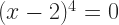
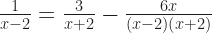
 , which turns our work into a linear equation. Very soon we find the solution must be
  . Which would make at least two of the denominators in the original equation zero. We know not to want that.
 . Although, before working out
  substitute that
  . Then we have


 we’re implicitly defining a function. A function has three pieces. It has a set called the domain, from which we draw the independent variable. It has a set called the range. It has a rule matching elements in the domain to an element in the range. We’ve only given the rule. What are the domain and what’s the range for
  ?
?  ? That can’t mean anything if x equals 2.
  would have a domain “real numbers other than 2 and -2”.
  to
to  by dividing out x is to cut
  out of the space of possible solutions.
  ? Rewrite that as a function.
  would seem to have a domain “x greater than or equal to 0”. The extraneous solution is
  , a number which rumor has it is greater than or equal to 0. What happened?
 on the right with
 and
and  .
.  has an implicit domain of “x greater than or equal to 0”. What’s the domain of
  ? If
? If  , like we said it does, then they have to agree for every x in either’s domain. So
  and
and  , you need their first derivatives,
  and
and  . If you have three functions,
  , you need first derivatives,
  , as well as second derivatives,
  ,
,  , and
, and  . If you have
  functions and here I’ll call them
  , you need
  derivatives,
  and so on through
  . You see right away this is a fun and exciting thing to calculate. Also why in intro to differential equations you only work this out with two or three functions. Maybe four functions if the class has been really naughty.
 ,
,  , and
, and  . Don’t know what they are; don’t care. The differential equation is a lot easier of
 that we want to find, is the same. It’s the right-hand-side that’s different, that’s a constant zero. This is what makes the new equation homogenous. This homogenous equation is easier and we can expect to find two functions,
  and
and  , that solve it. If
  . (The ‘p’ stands for ‘particular’, as in “the solution for this particular
  also has to solve that inhomogenous differential equation. It seems startling but if you work it out, it’s so. (The key is
  also has to solve that inhomogenous differential equation. In fact, for any constants
  and
and  , it has to be that
  is a solution.
 is the velocity. If we want to emphasize we think of vectors,
  is the position and
  the velocity.
  , or if we want to emphasize its vector nature,
  . Why a name besides the good enough
  , also known as
  . Or, if we’re sure we won’t lose a ‘ mark,
  . Once we are comfortable thinking of how position changes in time we can think of other changes. Velocity’s change in time we call acceleration. This is also a vector, more abstract than position or velocity. Multiply the acceleration by the mass of the thing accelerating and we have a vector called the “force”. That, we at least feel we understand, and can work with.
  , where n is some big enough number like 4.
  . The superscript-T there, “transposition”, lets us use the tools of matrix algebra. This vector describes a point in phase space. Phase space is the collection of all the physically possible positions and velocities for the system.
  , or,
, or,  . This acceleration itself depends on, normally, the positions and velocities. So we can describe this as
  for some function
  . You are surely impressed with this symbol-shuffling. You are less sure why this bother.
  . Or approximate our problem as a matrix problem. This lets us bring in linear algebra tools, and that’s worthwhile.
  . Most of them extend to
  . The result is a classic mathematician’s trick. We can recast a problem as one we have better tools to solve.
  , in the complex conjugate, that element would be
  . Reverse the plus or minus sign of the imaginary component. The shorthand for “the complex conjugate to matrix U” is
  . Also we’ll often just say “the conjugate”, taking the “complex” part as implied.
  .
.  . For a wonder, as matrices go, it doesn’t matter whether you take the transpose or the conjugate first. It’s the same
  . You may ask how people writing this out by hand never mistake
  . This is a good question and I hope to have an answer someday. (I would write it as
  in my notes.)
  .
.  for an identity matrix. If we have to be clear how many rows and columns the matrix has, we write that as a subscript:
  or
or  or
or  or so on.
  is a “diagonal” matrix. A diagonal matrix has zeroes for every element except the diagonal ones. That is, row one, column one; row two, column two; row three, column three; and so on. The elements that trace a path from the upper-left to the lower-right corner of the matrix. (The diagonal from the upper-right to the lower-left we have nothing to do with.) Everything we might do with matrices is easier on a diagonal matrix. So we process our matrix A into this diagonal matrix D. Process it by whatever the heck we’re doing. If we then multiply this by the inverses of U and V? If we calculate
  ? We get whatever our process would have given us had we done it to A. And, since U and V are unitary matrices, it’s easy to find these inverses. Wonderful!
  is a diagonal matrix. And then that’s great. The original H is hard to work with. The diagonalized version? That one we can almost always work with. And then we can go from solutions on the diagonalized version back to solutions on the original. (If the function
  describes the evolution of
  describes the evolution of
  .) The work that U (and
  . I don’t have a good way to describe what this is, physically; we can’t observe it directly. This symmetry, though, manifests as the conservation of electric charge, a thing we rather like.
  to
to  to
to  . That looks good, but then we have to ask: isn’t that just an operator? Also: then what about differential forms? Or
  is a quadratic form. So is
  ; the x times the y brings this to a second degree. Also a quadratic form is
  . So is
  .
.
 . Those of us who don’t do a lot of differential geometry think that looks funny. And we have more familiar ways to write things down. Like, we can put the collection of variables
  into an ordered
  into a square
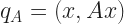
 , and the name “the equation of a circle”.
  is less familiar, but to the crowd reading this, not much less familiar. Fill that out to
  and we have a hyperbola. If we have
  and let that
  then we have an ellipse, something a bit wider than it is tall. Similarly
  is a hyperbola still, just anamorphic.
 just begs to equal
  . Or ellipsoids:
  , set equal to some (positive)
  or
or  , set equal to
  equalling some positive number describes a tube.)
 ? This also wants to be an ellipse.
 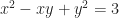 , to pick an easy number, is a rotated ellipse. The long axis is along the line described by
  . The short axis is along the line described by
  . How about — let me make this easy.
  ? The equation
  describes a hyperbola, but a rotated one, with the x- and y-axes
  might represent? If you’re thinking “ellipsoid, only it’s at an angle” you’re doing well. It runs really long in one direction, along the plane described by
  can, for sets of integers x, y, z, and w, add up to any positive number you like. (It’s not guaranteed this will happen.
  can’t produce 15.) We know of at least 54 combinations which generate all the positive integers, like
  and
and  and such.
 . I agree it looks nice. Particularly, though, we write
  , where f is some function. In practice, we’ll see functions like
  or
or  or
or  . Usually something simple like that. It can be tricky. There’s a scheme for multiplying large numbers together that’s
 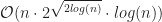 . What you will not see is something like
  , or
, or  or such. This comes to what we mean by the Big-O.
 ‘ is
‘ is  and
and  and
and  . The function ‘
 ‘ is also
  is right out.
 if, for every positive number C, whenever n is large enough g(n) is less than or equal to C times f(n). I know that sounds almost the same. Here’s why it’s not.
 . If g(n) is
  . But the function n is at least
  , and
, and  and those other fun variations. Being Little-O compels you to be Big-O. Big-O is not compelled to be Little-O, although it can happen.
 . Is it the case that for every positive number C it’s true that g(x) is less than C times f(x), once x is big enough? Then g(x) is
  .
. . We use this knowledge to make sure our error is tolerable. Also, we don’t usually care what the function is at x + h. It’s just what we can calculate. What we want is the function at some point a fair bit away from x, call it x + L. So we use our approximate knowledge of conditions at x + h to approximate the function at x + 2h. And use x + 2h to tell us about x + 3h, and from that x + 4h and so on, until we get to x + L. We’d like to have as few of these uninteresting intermediate points as we can, so look for as big an h as is safe.
 to be a tiny number. It seems odd to use the same notation with a large independent variable and with a small one. The concept carries over, though, and helps us talk efficiently about this different problem.


 to mean the sum of all l’s. By mid-November he was integrating functions, and writing out his work as
  . Any mathematics or physics or chemistry or engineering major today would recognize that. A year later he was writing things like
  , which we’d also understand if not quite care to put that way.
 and rewrite it as
  . Leibniz’s notation gives us the idea that taking derivatives is some kind of fraction. It isn’t, but in many problems we act as though it were. It works out often enough we forget that it might not.

 is parallelizable, ie, there exist n – 1 tangent vector fields to
  divides
  . There are only three values of ‘n’ that do that. For example.
  . Or you can have an ordered pair,
  . Or an ordered quadruple,
  . Or you can have an ordered octuple,
  . And that’s it. Not that other ordered sets can’t be interesting. They will all diverge far enough from the way real numbers work that you can’t do something that looks like division.
  and know what it meant. We won’t see that for any bigger ordered set of
  outside the stable range”. I know I don’t. I do know when I hear a beautiful string of syllables and that is a joy of mathematics never appreciated enough.
  . For every integer n we have the function
  where z is a real number between -π and π.
  then the Jacobi Polynomials are the Chebyshev Polynomials of the first kind. (There’s also a second kind.) These are handy in approximation theory, describing ways to better interpolate a polynomial from a set of data. They also have a neat, peculiar relationship to the multiple-cosine formulas. Like,
  . And the second Chebyshev polynomial is
  . Imagine sliding between x and
  and you see the relationship.
  and
and  . And so on.
 — you can find others. You do this in a way rather like how you find new terms in
  and
and  for the same α and β? Then you can calculate
  with nothing more than pen, paper, and determination. If it helps,

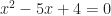 . That quadratic has two solutions, but it’s possible to have a quadratic with only one, such as
  . Or to have a quadratic with no solutions, such as, iconically,
  . We might underscore that by plotting the curve whose x- and y-coordinates makes true the equation
  . There’s no point on the curve with a y-coordinate of zero, so, there we go.
 and
and  . This is all right for introducing the idea that mathematics is a tool. If it doesn’t do something we need, we can alter it.
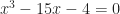 .
.
 for some real numbers a, b, and c, we’ve known about forever. Euclid solved these kinds of equations using geometric reasoning. Chinese mathematicians 2200 years ago described rules for how to find roots. The Indian mathematician Brahmagupta, by the early 7th century, described the quadratic formula to find at least one root. Both possible roots were known to Indian mathematicians a thousand years ago. We’ve reduced the formula today to
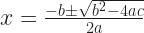
 . But stare at it and you can see where that’s “really” a quadratic pretending to be sixth-power. Finding there was no formula to find, though, lead people to develop group theory. And group theory underlies much of mathematics and modern physics.
 , came near the end of the 14th century in some manuscripts out of Florence. It’s built on a transformation. Transformations are key to mathematics. The point of a transformation is to turn a problem you don’t know how to do into one you do. As I write this, MathWorld lists 543 pages as matching “transformation”. That’s about half what “polynomial” matches (1,199) and about three times “trigonometric” (184). So that can help you judge importance.
 . And then figure out what
  and
and  are. Using all that, and the knowledge that
 . We would allow that p or q or both might be negative numbers.
 . This turns the depressed equation into
 and move things around a little. You get
 . Notice that’s the second of the three sorts of depressed polynomial. Cardano’s formula says that one of the roots will be at
![x = \sqrt[3]{\frac{q}{2} + r} + \sqrt[3]{\frac{q}{2} - r}](https://s0.wp.com/latex.php?latex=x+%3D+%5Csqrt%5B3%5D%7B%5Cfrac%7Bq%7D%7B2%7D+%2B+r%7D+%2B+%5Csqrt%5B3%5D%7B%5Cfrac%7Bq%7D%7B2%7D+-+r%7D+&bg=ffffff&fg=1a1a1a&s=2&c=20201002)

![x = \sqrt[3]{2 + \sqrt{-121}} + \sqrt[3]{2 - \sqrt{-121}}](https://s0.wp.com/latex.php?latex=x+%3D+%5Csqrt%5B3%5D%7B2+%2B+%5Csqrt%7B-121%7D%7D+%2B+%5Csqrt%5B3%5D%7B2+-+%5Csqrt%7B-121%7D%7D+&bg=ffffff&fg=1a1a1a&s=2&c=20201002)
 out of
  . What’s left is
  . You can use the quadratic formula for this. The other two roots are
  , about -0.268, and
  , about -3.732.
![R[x]/(x^2 + 1)](https://s0.wp.com/latex.php?latex=R%5Bx%5D%2F%28x%5E2+%2B+1%29+&bg=ffffff&fg=1a1a1a&s=0&c=20201002) . I don’t have the strength to explain all that today.
. I don’t have the strength to explain all that today. 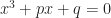 , rather than three. (Or more than three equations, if we have to work with an x we know to be negative.) Imaginary numbers we can start with, and find answers we know to be true. And this encourages us to find reasons to trust the results. Having one line of reasoning is good. Having several lines — Argand’s geometric, Hamilton’s coordinates, Cauchy’s rings — is reassuring. We may not be able to point to an imaginary number of anything. But if we can trust our arithmetic on real numbers we can trust our arithmetic on imaginary numbers.
 , instead of being called positive, negative, and imaginary (or worse still, impossible) unity, been given the names say, of direct, inverse, and lateral unity, there would hardly have been any scope for such obscurity”. I’ve never heard them term “impossible numbers”, except as an adjective.

 can describe you have tread in Lamé’s path.)
  was prime. This seems to be the largest prime number ever proven by hand. He also created the Tower of Hanoi problem.) In January of 1876, Lucas wrote about the Fibonacci sequence, describing it as “the series of Lamé”. By May, though in writing about prime numbers, he has read Boncompagni’s publications. He says how this thing “commonly known as the sequence of Lamé was first presented by Fibonacci”.
  and
and  and many other such exponential functions. One secret of algebra, not appreciated until calculus (or later), is that all these different functions are a single family. Understanding one exponential function lets you understand them all. Mathematicians pick one, the exponential with base e, because we find that convenient.
  .
. 
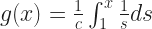

 but we already have
  in the works here. There is a limit to how many little one-stroke superscripts we need above g. This is the tradeoff to using ‘ for first derivatives. But here’s the important thing:
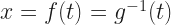


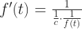


 for the correct value of c. Then all you need do is find a value of ‘c’ that makes that last equation true.
  . What is its velocity? That’s the first derivative of its position, so,
  .
.  is too small to notice. The motion declines into imperceptibility.
  .
.  , where
  and
and  are some real numbers whose value I don’t care about. What’s important here is that
  .
.  . This is an interesting complex number. Do you see what’s interesting about it? I’ll get there next paragraph.
  and
and  and
and  will all be
  for some real numbers a and b. In this case, you get spirals as t changes. If a is positive, you get points spiralling outward as t increases. If a is negative, you get points spiralling inward toward zero as t increases. If b is positive the spirals go counterclockwise. If b is negative the spirals go clockwise.
  is the same as
  .
.  , is equal to the product of the exponential of those terms. This is a good thing to have in your portfolio. If I remember right, it comes in around the 25th thing. It’s an easy result to have if you already showed something about the logarithms of products.
  , though.
  ? How about a
  ? Maybe something else? An arc-cosine of
  ? Here, and later on, a and b and c are some real numbers.
  means “multiply the real number b by whatever
  . And if you just try that, with
  . Mathematicians do this so often it can take a moment to remember that is just a convention. And there is a common matching between points in a Cartesian coordinate system and vectors. Chaining together matches like this can worry. Trust that we believe our matches are sound. Then we notice that adding two complex numbers does the same work as adding ordered coordinate pairs. If we trust that adding coordinate pairs makes sense, then we need to accept that adding complex numbers makes sense. Adding coordinate pairs is the same work as adding real numbers. It’s just a lot of them. So we’re lead to trust that if addition for real numbers works then addition for complex numbers does.
  . Let the second have polar coordinates
  . Their product, by the rules of complex numbers, is a point with polar coordinates
  . These polar coordinates are real numbers again. If we trust addition and multiplication of real numbers, we can trust this for complex numbers.
 ![a \left[\begin{tabular}{c c} 1 & 0 \\ 0 & 1 \end{tabular}\right] + b \left[\begin{tabular}{c c} 0 & 1 \\ -1 & 0 \end{tabular}\right]](https://s0.wp.com/latex.php?latex=a+%5Cleft%5B%5Cbegin%7Btabular%7D%7Bc+c%7D+1+%26+0+%5C%5C+0+%26+1+%5Cend%7Btabular%7D%5Cright%5D+%2B+b+%5Cleft%5B%5Cbegin%7Btabular%7D%7Bc+c%7D+0+%26+1+%5C%5C+-1+%26+0++%5Cend%7Btabular%7D%5Cright%5D++&bg=ffffff&fg=1a1a1a&s=2&c=20201002)


![Comic strip Chaos Butterfly Man: 'Bitten by a radioactive chaos butterfly, Mike Mason gained the powers of a chaos butterfly!' [ Outside a bank ] Mason flaps his arm at an escaping robber. Robber: 'Ha-ha! What harm can THAT do me?' [ Nine days later ] Robber: 'Where did this thunderstorm finally come fr ... YOW!' (He's struck by lightning.)](https://nebusresearch.wordpress.com/wp-content/uploads/2020/06/super-fun-pak-comics_ruben-bolling_23-may-2020.gif)
