My All 2020 Mathematics A to Z: J Willard Gibbs

Charles Merritt sugested a biographical subject for G. (There are often running themes in an A-to-Z and this year’s seems to be “biography”.) I don’t know of a web site or other project that Merritt has that’s worth sharing, but if I learn of it, I’ll pass it along.

Color cartoon illustration of a coati in a beret and neckerchief, holding up a director's megaphone and looking over the Hollywood hills. The megaphone has the symbols + x (division obelus) and = on it. The Hollywood sign is, instead, the letters MATHEMATICS. In the background are spotlights, with several of them crossing so as to make the letters A and Z; one leg of the spotlights has 'TO' in it, so the art reads out, subtly, 'Mathematics A to Z'. — Art by Thomas K Dye, creator of the web comics **Projection Edge**, **Newshounds**, **Infinity Refugees**, and **Something Happens**. He’s on Twitter as @projectionedge. You can get to read **Projection Edge** six months early by subscribing to his Patreon.

J Willard Gibbs.

My love and I, like many people, tried last week to see the comet NEOWISE. It took several attempts. When finally we had binoculars and dark enough sky we still had the challenge of where to look. Finally determined searching and peripheral vision (which is more sensitive to faint objects) found the comet. But how to guide the other to a thing barely visible except with binoculars? Between the silhouettes of trees and a convenient pair of guide stars we were able to put the comet’s approximate location in words. Soon we were experts at finding it. We could turn a head, hold up the binoculars, and see a blue-ish puff of something.

To perceive a thing is not to see it. Astronomy is full of things seen but not recognized as important. There is a great need for people who can describe to us how to see a thing. And this is part of the significance of J Willard Gibbs.

American science, in the 19th century, had an inferiority complex compared to European science. Fairly, to an extent: what great thinkers did the United States have to compare to William Thompson or Joseph Fourier or James Clerk Maxwell? The United States tried to argue that its thinkers were more practical minded, with Joseph Henry as example. Without downplaying Henry’s work, though? The stories of his meeting the great minds of Europe are about how he could fix gear that Michael Faraday could not. There is a genius in this, yes. But we are more impressed by magnetic fields than by any electromagnet.

Gibbs is the era’s exception, a mathematical physicist of rare insight and creativity. In his ability to understand problems, yes. But also in organizing ways to look at problems so others can understand them better. A good comparison is to Richard Feynman, who understood a great variety of problems, and organized them for other people to understand. No one, then or now, doubted Gibbs compared well to the best European minds.

Gibbs’s life story is almost the type case for a quiet academic life. He was born into an academic/ministerial family. Attended Yale. Earned what appears to be the first PhD in engineering granted in the United States, and only the fifth non-honorary PhD in the country. Went to Europe for three years, then came back home, got a position teaching at Yale, and never left again. He was appointed Professor of Mathematical Physics, the first such in the country, at age 32 and before he had even published anything. This speaks of how well-connected his family was. Also that he was well-off enough not to need a salary. He wouldn’t take one until 1880, when Yale offered him two thousand per year against Johns Hopkins’s three.

Between taking his job and taking his salary, Gibbs took time to remake physics. This was in thermodynamics, possibly the most vibrant field of 19th century physics. The wonder and excitement we see in quantum mechanics resided in thermodynamics back then. Though with the difference that people with a lot of money were quite interested in the field’s results. These were people who owned railroads, or factories, or traction companies. Extremely practical fields.

What Gibbs offered was space, particularly, phase space. Phase space describes the state of a system as a point in … space. The evolution of a system is typically a path winding through space. Constraints, like the conservation of energy, we can usually understand as fixing the system to a surface in phase space. Phase space can be as simple as “the positions and momentums of every particle”, and that often is what we use. It doesn’t need to be, though. Gibbs put out diagrams where the coordinates were things like temperature or pressure or entropy or energy. Looking at these can let one understand a thermodynamic system. They use our geometric sense much the same way that charts of high- and low-pressure fronts let one understand the weather. James Clerk Maxwell, famous for electromagnetism, was so taken by this he created plaster models of the described surface.

This is, you might imagine, pretty serious, heady stuff. So you get why Gibbs published it in the Transactions of the Connecticut Academy: his brother-in-law was the editor. It did not give the journal lasting fame. It gave his brother-in-law a heightened typesetting bill, and Yale faculty and New Haven businessmen donated funds.

Which gets to the less-happy parts of Gibbs’s career. (I started out with ‘less pleasant’ but it’s hard to spot an actually unpleasant part of his career.) This work sank without a trace, despite Maxwell’s enthusiasm. It emerged only in the middle of the 20th century, as physicists came to understand their field as an expression of geometry.

That’s all right. Chemists understood the value of Gibbs’s thermodynamics work. He introduced the enthalpy, an important thing that nobody with less than a Master’s degree in Physics feels they understand. Changes of enthalpy describe how heat transfers. And the Gibbs Free Energy, which measures how much reversible work a system can do if the temperature and pressure stay constant. A chemical reaction where the Gibbs free energy is negative will happen spontaneously. If the system’s in equilibrium, the Gibbs free energy won’t change. (I need to say the Gibbs free energy as there’s a different quantity, the Helmholtz free energy, that’s also important but not the same thing.) And, from this, the phase rule. That describes how many independently-controllable variables you can see in mixing substances.

In the 1880s Gibbs worked on something which exploded through physics and mathematics. This was vectors. He didn’t create them from nothing. Hermann Günter Grassmann — whose fascinating and frustrating career I hadn’t known of before this — laid much of the foundation. Building on Grassman and W K Clifford, though, let Gibbs present vectors as we now use them in physics. How to define dot products and cross products. How to use them to simplify physics problems. How they’re less work than quaternions are. Gibbs was not the only person to recast physics in vector form. Oliver Heaviside is another important mathematical physicist of the time who did. But Gibbs identified the tools extremely well. You can read his Elements of Vector Analysis. It’s not very different from what a modern author would write on the subject. It’s terser than I would write, but terse is also respectful of someone’s time and ability to reason out explanations of small points.

There are more pieces. They don’t all fit in a neat linear timeline; nobody’s life really does. Gibbs’s thermodynamics work, leading into statistical mechanics, foreshadows much of quantum mechanics. He’s famous for the Gibbs Paradox, which concerns the entropy of mixing together two different kinds of gas. Why is this different from mixing together two containers of the same kind of gas? And the answer is that we have to think more carefully about what we mean by entropy, and about the differences between containers.

There is a Gibbs phenomenon, known to anyone studying Fourier series. The Fourier series is a sum of sine and cosine functions. It approximates an arbitrary original function. The series is a continuous function; you could draw it without lifting your pen. If the original function has a jump, though? A spot where you have to lift your pen? The Fourier series for that represents the jump with a region where its quite-good approximation suddenly turns bad. It wobbles around the ‘correct’ values near the jump. Using more terms in the series doesn’t make the wobbling shrink. Gibbs described it, in studying sawtooth waves. As it happens, Henry Wilbraham first noticed and described this in 1848. But Wilbraham’s work went unnoticed until after Gibbs’s rediscovery.

And then there was a bit in which Gibbs was intrigued by a comet that prolific comet-spotter Lewis Swift observed in 1880. Finding the orbit of a thing from a handful of observations is one of the great problems of astronomical mathematics. Karl Friedrich Gauss started the 19th century with his work projecting the orbit of the newly-discovered and rapidly-lost asteroid Ceres. Gibbs put his vector notation to the work of calculating orbits. His technique, I am told by people who seem to know, is less difficult and more numerically stable than was earlier used.

Swift’s comet of 1880, it turns out, was spotted in 1869 by Wilhelm Tempel. It was lost after its 1908 perihelion. Comets have a nasty habit of changing their orbits on us. But it was rediscovered in 2001 by the Lincoln Near-Earth Asteroid Research program. It’s next to reach perihelion the 26th of November, 2020. You might get to see this, another thing touched by J Willard Gibbs.

This and the other other A-to-Z topics for 2020 should be at this link. All my essays for this and past A-to-Z sequences are at this link. I’ll soon be opening f or topics for J, K, and L, essays also. Thanks for reading.

My 2019 Mathematics A To Z: Buffon’s Needle

Today’s A To Z term was suggested by Peter Mander. Mander authors CarnotCycle, which when I first joined WordPress was one of the few blogs discussing thermodynamics in any detail. When I last checked it still was, which is a shame. Thermodynamics is a fascinating field. It’s as deeply weird and counter-intuitive and important as quantum mechanics. Yet its principles are as familiar as a mug of warm tea on a chilly day. Mander writes at a more technical level than I usually do. But if you’re comfortable with calculus, or if you’re comfortable nodding at a line and agreeing that he wouldn’t fib to you about a thing like calculus, it’s worth reading.

Cartoony banner illustration of a coati, a raccoon-like animal, flying a kite in the clear autumn sky. A skywriting plane has written 'MATHEMATIC A TO Z'; the kite, with the letter 'S' on it to make the word 'MATHEMATICS'. — Art by Thomas K Dye, creator of the web comics **Projection Edge**, **Newshounds**, **Infinity Refugees**, and **Something Happens**. He’s on Twitter as @projectionedge. You can get to read **Projection Edge** six months early by subscribing to his Patreon.

Buffon’s Needle.

I’ve written of my fondness for boredom. A bored mind is not one lacking stimulation. It is one stimulated by anything, however petty. And in petty things we can find great surprises.

I do not know what caused Georges-Louis Leclerc, Comte de Buffon, to discover the needle problem named for him. It seems like something born of a bored but active mind. Buffon had an active mind: he was one of Europe’s most important naturalists of the 1700s. He also worked in mathematics, and astronomy, and optics. It shows what one can do with an engaged mind and a large inheritance from one’s childless uncle who’s the tax farmer for all Sicily.

The problem, though. Imagine dropping a needle on a floor that has equally spaced parallel lines. What is the probability that the needle will land on any of the lines? It could occur to anyone with a wood floor who’s dropped a thing. (There is a similar problem which would occur to anyone with a tile floor.) They have only to be ready to ask the question. Buffon did this in 1733. He had it solved by 1777. We, with several centuries’ insight into probability and calculus, need less than 44 years to solve the question.

Let me use L as the length of the needle. And d as the spacing of the parallel lines. If the needle’s length is less than the spacing then this is an easy formula to write, and not too hard to calculate. The probability, P, of the needle crossing some line is:

$P = \frac{2}{\pi}\frac{L}{d}$

I won’t derive it rigorously. You don’t need me for that. The interesting question is whether this formula makes sense. That L and d are in it? Yes, that makes sense. The length of the needle and the gap between lines have to be in there. More, the probability has to have the ratio between the two. There’s different ways to argue this. Dimensional analysis convinces me, at least. Probability is a pure number. L is a measurement of length; d is a measurement of length. To get a pure number starting with L and d means one of them has to divide into the other. That L is in the numerator and d the denominator makes sense. A tiny needle has a tiny chance of crossing a line. A large needle has a large chance. That $\frac{L}{d}$ is raised to the first power, rather than the second or third or such … well, that’s fair. A needle twice as long having twice the chance of crossing a line? That sounds more likely than a needle twice as long having four times the chance, or eight times the chance.

Does the 2 belong there? Hard to say. 2 seems like a harmless enough number. It appears in many respectable formulas. That π, though …

That π …

π comes to us from circles. We see it in calculations about circles and spheres all the time. We’re doing a problem with lines and line segments. What business does π have showing up?

We can find reasons. One way is to look at a similar problem. Imagine dropping a disc on these lines. What’s the chance the disc falls across some line? That’s the chance that the center of the disc is less than one radius from any of the lines. What if the disc has an equal chance of landing anywhere on the floor? Then it has a probability of $\frac{L}{d}$ of crossing a line. If the radius is smaller than the distance between lines, anyway. If the radius is larger than that, the probability is 1.

Now draw a diameter line on this disc. What’s the chance that this diameter line crosses this floor line? That depends on a couple things. Whether the center of the disc is near enough a floor line. And what angle the diameter line makes with respect to the floor lines. If the diameter line is parallel the floor line there’s almost no chance. If the diameter line is perpendicular to the floor line there’s the best possible chance. But that angle might be anything.

Let me call that angle θ. The diameter line crosses the floor line if the diameter times the sine of θ is less than half the distance between floor lines. … Oh. Sine. Sine and cosine and all the trigonometry functions we get from studying circles, and how to draw triangles within circles. And this diameter-line problem looks the same as the needle problem. So that’s where π comes from.

I’m being figurative. I don’t think one can make a rigorous declaration that the π in the probability formula “comes from” this sine, any more than you can declare that the square-ness of a shape comes from any one side. But it gives a reason to believe that π belongs in the probability.

If the needle’s longer than the gap between floor lines, if $L > d$ , there’s still a probability that the needle crosses at least one line. It never becomes certain. No matter how long the needle is it could fall parallel to all the floor lines and miss them all. The probability is instead:

$P = \frac{2}{\pi}\left(\frac{L}{d} - \sqrt{\left(\frac{L}{d}\right)^2 - 1} + \sec^{-1}\left(\frac{L}{d}\right)\right)$

Here $\sec^{-1}$ is the world-famous arcsecant function. That is, it’s whatever angle has as its secant the number $\frac{L}{d}$ . I don’t mean to insult you. I’m being kind to the person reading this first thing in the morning. I’m not going to try justifying this formula. You can play with numbers, though. You’ll see that if $\frac{L}{d}$ is a little bit bigger than 1, the probability is a little more than what you get if $\frac{L}{d}$ is a little smaller than 1. This is reassuring.

The exciting thing is arithmetic, though. Use the probability of a needle crossing a line, for short needles. You can re-write it as this:

$\pi = 2\frac{L}{d}\frac{1}{P}$

L and d you can find by measuring needles and the lines. P you can estimate. Drop a needle many times over. Count how many times you drop it, and how many times it crosses a line. P is roughly the number of crossings divided by the number of needle drops. Doing this gives you a way to estimate π. This gives you something to talk about on Pi Day.

It’s a rubbish way to find π. It’s a lot of work, plus you have to sweep needles off the floor. Well, you can do it in simulation and avoid the risk of stepping on an overlooked needle. But it takes a lot of needle-drops to get good results. To be certain you’ve calculated the first two decimal points correctly requires 3,380,000 needle-drops. Yes, yes. You could get lucky and happen to hit on an estimate of 3.14 for π with fewer needle-drops. But if you were sincerely trying to calculate the digits of π this way? If you did not know what they were? You would need the three and a third million tries to be confident you had the number correct.

So this result is, as a practical matter, useless. It’s a heady concept, though. We think casually of randomness as … randomness. Unpredictability. Sometimes we will speak of the Law of Large Numbers. This is several theorems in probability. They all point to the same result. That if some event has (say) a probability of one-third of happening, then given 30 million chances, it will happen quite close to 10 million times.

This π result is another casting of the Law of Large Numbers, and of the apparent paradox that true unpredictability is itself predictable. There is no way to predict whether any one dropped needle will cross any line. It doesn’t even matter whether any one needle crosses any line. An enormous number of needles, tossed without fear or favor, will fall in ways that embed π. The same π you get from comparing the circumference of a circle to its diameter. The same π you get from looking at the arc-cosine of a negative one.

I suppose we could use this also to calculate the value of 2, but that somehow seems to touch lesser majesties.

Thank you again for reading. All of the Fall 2019 A To Z posts should be at this link. This year’s and all past A To Z sequences should be at this link. I’ve made my picks for next week’s topics, and am fooling myself into thinking I have a rough outline for them already. But I’m still open for suggestions for the letters E through H and appreciate suggestions.

Particle Physics Made Hard

A friend was playing with that cute little particle-physics simulator idea I mentioned last week. And encountered a problem. With a little bit of thought, I was able to not solve the problem. But I was able to explain why it was a subtler and more difficult problem than they had realized. These are the moments that make me feel justified calling myself a mathematician.

The proposed simulation was simple enough: imagine a bunch of particles that interact by rules that aren’t necessarily symmetric. Like, the attraction particle A exerts on particle B isn’t the same as what B exerts on A. Or there are multiple species of particles. So (say) red particles are attracted to blue but repelled by green. But green is attracted to red and repelled by blue twice as strongly as red is attracted to blue. Your choice.

Give a mathematician a perfectly good model of something. She’ll have the impulse to try tinkering with it. One reliable way to tinker with it is to change the domain on which it works. If your simulation supposes you have particles moving on the plane, then, what if they were in space instead? Or on the surface of a sphere? Or what if something was strange about the plane? My friend had this idea: what if the particles were moving on the surface of a cube?

And the problem was how to find the shortest distance between two particles on the surface of a cube. The distance matters since most any attraction rule depends on the distance. This may be as simple as “particles more than this distance apart don’t interact in any way”. The obvious approach, or if you prefer the naive approach, is to pretend the cube is a sphere and find distances that way. This doesn’t get it right, not if the two points are on different faces of the cube. If they’re on adjacent faces, ones which share an edge — think the floor and the wall of a room — it seems straightforward enough. My friend got into trouble with points on opposite faces. Think the floor and the ceiling.

This problem was posed (to the public) in January 1905 by Henry Ernest Dudeney. Dudeney was a newspaper columnist with an exhaustive list of mathematical puzzles. A couple of the books collecting them are on Project Gutenberg. The puzzles show their age in spots. Some in language; some in problems that ask to calculate money in pounds-shillings-and-pence. Many of them are chess problems. But many are also still obviously interesting, and worth thinking about. This one, I was able to find, was a variation of The Spider and the Fly, problem 75 in The Canterbury Puzzles:

Inside a rectangular room, measuring 30 feet in length and 12 feet in width and height, a spider is at a point on the middle of one of the end walls, 1 foot from the ceiling, as at A; and a fly is on the opposite wall, 1 foot from the floor in the centre, as shown at B. What is the shortest distance that the spider must crawl in order to reach the fly, which remains stationary? Of course the spider never drops or uses its web, but crawls fairly.

(Also I admire Dudeney’s efficient closing off of the snarky, problem-breaking answer someone was sure to give. It suggests experienced thought about how to pose problems.)

What makes this a puzzle, even a paradox, is that the obvious answer is wrong. At least, what seems like the obvious answer is to start at point A, move to one of the surfaces connecting the spider’s and the fly’s starting points, and from that move to the fly’s surface. But, no: you get a shorter answer by using more surfaces. Going on a path that seems like it wanders more gets you a shorter distance. The solution’s presented here, along with some follow-up problems. In this case, the spider’s shortest path uses five of the six surfaces of the room.

The approach to finding this is an ingenious one. Imagine the room as a box, and unfold it into something flat. Then find the shortest distance on that flat surface. Then fold the box back up. It’s a good trick. It turns out to be useful in many problems. Mathematical physicists often have reason to ponder paths of things on flattenable surfaces like this. Sometimes they’re boxes. Sometimes they’re toruses, the shape of a doughnut. This kind of unfolding often makes questions like “what’s the shortest distance between points” easier to solve.

There are wrinkles to the unfolding. Of course there are. How interesting would it be if there weren’t? The wrinkles amount to this. Imagine you start at the corner of the room, and walk up a wall at a 45 degree angle to the horizon. You’ll get to the far corner eventually, if the room has proportions that allow it. All right. But suppose you walked up at an angle of 30 degrees to the horizon? At an angle of 75 degrees? You’ll wind your way around the walls (and maybe floor and ceiling) some number of times, each path you start with. Probably different numbers of times. Some path will be shortest, and that’s fine. But … like, think about the path that goes along the walls and ceiling and floor three times over. The room, unfolded into a flat panel, has only one floor and one ceiling and each wall once. The straight line you might be walking goes right off the page.

And this is the wrinkle. You might need to tile the room. In a column of blocks (like in Dudeney’s solution) every fourth block might be the floor, with, between any two of them, a ceiling. This is fine, and what’s needed. It can be a bit dizzying to imagine such a state of affairs. But if you’ve ever zoomed a map of the globe out far enough that you see Australia six times over then you’ve understood how this works.

I cannot attest that this has helped my friend in the slightest. I am glad that my friend wanted to think about the surface of the cube. The surface of a dodecahedron would be far, far past my ability to help with.

A Neat Fake Particle Physics Simulator

A friend sent me this video, after realizing that I had missed an earlier mention of it and thought it weird I never commented on it. And I wanted to pass it on, partly because it’s neat and partly because I haven’t done enough writing about topics besides the comics recently.

Particle Life: A Game Of Life Made Of Particles is, at least in video form, a fascinating little puzzle. The Game of Life referenced is one that anybody reading a pop mathematics blog is likely to know. But here goes. The Game of Life is this iterative process. We look at a grid of points, with each point having one of a small set of possible states. Traditionally, just two. At each iteration we go through every grid location. We might change that state. Whether we do depends on some simple rules. In the original Game of Life it’s (depending on your point of view) two or either three rules. A common variation is to include “mutations”, where a location’s state changes despite what the other rules would dictate. And the fascinating thing is that these very simple rules can yield incredibly complicated and beautiful patterns. It’s a neat mathematical refutation of the idea that life is so complicated that it must take a supernatural force to generate. It turns out that many things following simple rules can produce complicated patterns. We will often call them “unpredictable”, although (unless we do have mutations) they are literally perfectly predictable. They’re just chaotic, with tiny changes in the starting conditions often resulting in huge changes in behavior quickly.

This Particle Life problem is built on similar principles. The model is different. Instead of grid locations there are a cloud of particles. The rules are a handful of laws of attraction-or-repulsion. That is, that each particle exerts a force on all the other particles in the system. This is very like the real physics, of clouds of asteroids or of masses of electrically charged gasses or the like. But, like, a cloud of asteroids has everything following the same rule, everything attracts everything else with an intensity that depends on their distance apart. Masses of charged particles follow two rules, particles attracting or repelling each other with an intensity that depends on their distance apart.

This simulation gets more playful. There can be many kinds of particles. They can follow different and non-physically-realistic rules. Like, a red particle can be attracted to a blue, while a blue particle is repelled by a red. A green particle can be attracted to a red with twice the intensity that a red particle’s attracted to a green. Whatever; set different rules and you create different mock physics.

The result is, as the video shows, particles moving in “unpredictable” ways. Again, here, it’s “unpredictable” in the same way that I couldn’t predict when my birthday will next fall on a Tuesday. That is to say, it’s absolutely predictable; it’s just not obvious before you do the calculations. Still, it’s wonderful watching and tinkering with, if you have time to create some physics simulators. There’s source code for one in C++ that you might use. If you’re looking for little toy projects to write on your own, I suspect this would be a good little project to practice your Lua/LOVE coding, too.

Reading the Comics, April 5, 2019: The Slow Week Edition

People reading my Reading the Comics post Sunday maybe noticed something. I mean besides my correct, reasonable complaining about the Comics Kingdom redesign. That is that all the comics were from before the 30th of March. That is, none were from the week before the 7th of April. The last full week of March had a lot of comic strips. The first week of April didn’t. So things got bumped a little. Here’s the results. It wasn’t a busy week, not when I filter out the strips that don’t offer much to write about. So now I’m stuck for what to post Thursday.

Jason Poland’s Robbie and Bobby for the 3rd is a Library of Babel comic strip. This is mathematical enough for me. Jorge Luis Borges’s Library is a magnificent representation of some ideas about infinity and probability. I’m surprised to realize I haven’t written an essay specifically about it. I have touched on it, in writing about normal numbers, and about the infinite monkey theorem.

At a tower. Bobby: 'The library of Babel!' Robbie: 'Inside is every book that will ever be written! It may take the rest of our lives to search, but it'll be worth it!' Bobby: 'What? No index?' Robbie: 'The search for meaning has no index.' Bobby (on the phone): 'I just downloaded one.' Robbie: 'It can't have everything. ... Mark Twain vs Frankenstein? Dante in Space? Harry Potter Infinity?' Bobby: 'Yep. All available as e-books too! Wow, Jeff Goldblum does the audio books.' Robbie: 'pfff. Well, forget this place!' (They leave a 'BORING' sign across the library's door.) — Jason Poland’s **Robbie and Bobby** for the 3rd of April, 2019. I would have sworn that I write more about this strip. But this seems to be the first time I’ve mentioned it since 2017. Well, that and other **Robbie and Bobby**-based essays are at this link.

The strip explains things well enough. The Library holds every book that will ever be written. In the original story there are some constraints. Particularly, all the books are 410 pages. If you wanted, say, a 600-page book, though, you could find one book with the first 410 pages and another book with the remaining 190 pages and then some filler. The catch, as explained in the story and in the comic strip, is finding them. And there is the problem of finding a ‘correct’ text. Every possible text of the correct length should be in there. So every possible book that might be titled Mark Twain vs Frankenstein, including ones that include neither Mark Twain nor Frankenstein, is there. Which is the one you want to read?

Over a pizza. Reggie: 'Don't let Jughead near the pizza! He always ends up eating half of it!' Jughead, with the cutter: 'Relax! I've divided it into four equal slices! Check it yourself!' Reggie: 'OK, I guess they do look equal.' Archie: 'Except for one thing! There are only three of us!' (Reggie and Archie each have one slice; Jughead has two.) — Henry Scarpelli and Craig Boldman’s **Archie** for the 4th of April, 2019. Now this strip I’ve written about as recently as October. That appearance, and other **Archie** strips, are discussed at this link.

Henry Scarpelli and Craig Boldman’s Archie for the 4th features an equal-divisions problem. In principle, it’s easy to divide a pizza (or anything else) equally; that’s what we have fractions for. Making them practical is a bit harder. I do like Jughead’s quick work, though. It’s got the slight-of-hand you expect from stage magic.

Caterpillars in an algebra classroom. On the back of one caterpillar student is a sign, 'Kick^{10} me'. — Scott Hilburn’s **The Argyle Sweater** for the 4th of April, 2019. And this strip I’ve written about … wait, can I really have gone since early March without mentioning? Huh. Well, so it appears. Essays discussing **The Argyle Sweater** appear at this link.

Scott Hilburn’s The Argyle Sweater for the 4th takes place in an algebra class. I’m not sure what algebraic principle $7^4 \times 13^6$ demonstrates, but it probably came from somewhere. It’s 4,829,210. The exponentials on the blackboard do cue the reader to the real joke, of the sign reading “kick¹⁰ me”. I question whether this is really an exponential kicking situation. It seems more like a simple multiplication to me. But it would be harder to make that joke read clearly.

Tony Cochran’s Agnes for the 5th is part of a sequence investigating how magnets work. Agnes and Trout find just … magnet parts inside. This is fair. It’s even mathematics.

Looking over a pile of debris and a hammer on the table. Agnes: 'OK, we smashed a magnet. What do we see?' Trout: 'Uh. Magnet crumbs.' Agnes: 'Me too. I see magnet crumbs.' Trout: 'No gizmos, no gears, no wires. Just dirty black magnet crumbs.' Agnes: 'So what does this tell us about magnet function?' Trout: 'That it's one of God's many mysteries. Let's go eat.' — Tony Cochran’s **Agnes** for the 5th of April, 2019. And this strip I quite like, but don’t get to discuss enough. My essays featuring **Agnes** appears at this link.

Thermodynamics classes teach one of the great mathematical physics models. This is about what makes magnets. Magnets are made of … smaller magnets. This seems like question-begging. Ultimately you get down to individual molecules, each of which is very slightly magnetic. When small magnets are lined up in the right way, they can become a strong magnet. When they’re lined up in another way, they can be a weak magnet. Or no magnet at all.

How do they line up? It depends on things, including how the big magnet is made, and how it’s treated. A bit of energy can free molecules to line up, making a stronger magnet out of a weak one. Or it can break up the alignments, turning a strong magnet into a weak one. I’ve had physics instructors explain that you could, in principle, take an iron rod and magnetize it just by hitting it hard enough on the desk. And then demagnetize it by hitting it again. I have never seen one do this, though.

This is more than just a physics model. The mathematics of it is … well, it can be easy enough. A one-dimensional, nearest-neighbor model, lets us describe how materials might turn into magnets or break apart, depending on their temperature. Two- or three-dimensional models, or models that have each small magnet affected by distant neighbors, are harder.

And then there’s the comic strips that didn’t offer much to write about.
Brian Basset’s Red and Rover for the 3rd,
Liniers’s Macanudo for the 5th, Stephen Bentley’s Herb and Jamaal rerun for the 5th, and Gordon Bess’s Redeye rerun for the 5th all idly mention mathematics class, or things brought up in class.

Doug Savage’s Savage Chickens for the 2nd is another more-than-100-percent strip. Richard Thompson’s Richard’s Poor Almanac for the 3rd is a reprint of his Christmas Tree guide including a fir that “no longer inhabits Euclidean space”.

Mike Baldwin’s Cornered for the 31st depicts a common idiom about numbers. Eric the Circle for the 5th, by Rafoliveira, plays on the ∞ symbol.

And that covers the mathematically-themed comic strips from last week. There are more coming, though. I’ll show them on Sunday. Thanks for reading.

My 2018 Mathematics A To Z: Sorites Paradox

Today’s topic is the lone (so far) request by bunnydoe, so I’m under pressure to make it decent. If she or anyone else would like to nominate subjects for the letters U through Z, please drop me a note at this post. I keep fooling myself into thinking I’ll get one done in under 1200 words.

Cartoon of a thinking coati (it's a raccoon-like animal from Latin America); beside him are spelled out on Scrabble titles, 'MATHEMATICS A TO Z', on a starry background. Various arithmetic symbols are constellations in the background. — Art by Thomas K Dye, creator of the web comics **Newshounds**, **Something Happens**, and **Infinity Refugees**. His current project is **Projection Edge**. And you can get Projection Edge six months ahead of public publication by subscribing to his Patreon. And he’s on Twitter as @Newshoundscomic.

Sorites Paradox.

This is a story which makes a capitalist look kind of good. I say nothing about its truth, or even, at this remove, where I got it. The story as I heard it was about Ray Kroc, who made McDonald’s into a thing people of every land can complain about. The story has him demonstrate skepticism about the use of business consultants. A consultant might find, for example, that each sesame-seed hamburger bun has (say) 43 seeds. And that if they just cut it down to 41 seeds then each franchise would save (say) $50,000 annually. And no customer would notice the difference. Fine; trim the seeds a little. The next round of consultant would point out, cutting from 41 seeds to 38 would save a further $65,000 per store per year. And again no customer would notice the difference. Cut to 36 seeds? No customer would notice. This process would end when each bun had three sesame seeds, and the customers notice.

I mention this not for my love of sesame-seed buns. It’s just a less-common version of the Sorites Paradox. It’s a very old logical problem. We draw it, and its name, from the Ancient Greek philosophers. In the oldest form, it’s about a heap of sand, and which grain of sand’s removal destroys the heap. This form we attribute to Eubulides of Miletus. Eubulides is credited with a fair number of logical paradoxes. One of them we all know, the Liar Paradox, “What I am saying now is a lie”. Another, the Horns Paradox, I hadn’t encountered before researching this essay. But it bids fair to bring me some delight every day of the rest of my life. “What you have not lost, you have. But you have not lost horns. Therefore you have horns.” Eubelides has a bunch of other paradoxes. Some read, to my uninformed eye, like restatements of other paradoxes. Some look ready to be recast as arguments about Lois Lane’s relationship with Superman. Miletus we know because for a good stretch there every interesting philosopher was hanging around Miletus.

Part of the paradox’s intractability must be that it’s so nearly induction. Induction is a fantastic tool for mathematical problems. We couldn’t do without it. But consider the argument. If a bun is unsatisfying, one more seed won’t make it satisfying. A bun with one seed is unsatisfying. Therefore all buns have an unsatisfying number of sesame seeds on them. It suggests there must be some point at which “adding one more seed won’t help” stops being true. Fine; where is that point, and why isn’t it one fewer or one more seed?

A certain kind of nerd has a snappy answer for the Sorites Paradox. Test a broad population on a variety of sesame-seed buns. There’ll be some so sparse that nearly everyone will say they’re unsatisfying. There’ll be some so abundant most everyone agrees they’re great. So there’s the buns most everyone says are fine. There’s the buns most everyone says are not. The dividing line is at any point between the sparsest that satisfy most people and the most abundant that don’t. The nerds then declare the problem solved and go off. Let them go. We were lucky to get as much of their time as we did. They’re quite busy solving what “really” happened for Rashomon. The approach of “set a line somewhere” is fine if all want is guidance on where to draw a line. It doesn’t help say why we can anoint some border over any other. At least when we use a river as border between states we can agree going into the water disrupts what we were doing with the land. And even then we have to ask what happens during droughts and floods, and if the river is an estuary, how tides affect matters.

We might see an answer by thinking more seriously about these sesame-seed buns. We force a problem by declaring that every bun is either satisfying or it is not. We can imagine buns with enough seeds that we don’t feel cheated by them, but that we also don’t feel satisfied by. This reflects one of the common assumptions of logic. Mathematicians know it as the Law of the Excluded Middle. A thing is true or it is not true. There is no middle case. This is fine for logic. But for everyday words?

It doesn’t work when considering sesame-seed buns. I can imagine a bun that is not satisfying, but also is not unsatisfying. Surely we can make some logical provision for the concept of “meh”. Now we need not draw some arbitrary line between “satisfying” and “unsatisfying”. We must draw two lines, one of them between “unsatisfying” and “meh”. There is a potential here for regression. Also for the thought of a bun that’s “satisfying-meh-satisfying by unsatisfying”. I shall step away from this concept.

But there are more subtle ways to not exclude the middle. For example, we might decide a statement’s truth exists on a spectrum. We can match how true a statement is to a number. Suppose an obvious falsehood is zero; an unimpeachable truth is one, and normal mortal statements somewhere in the middle. “This bun with a single sesame seed is satisfying” might have a truth of 0.01. This perhaps reflects the tastes of people who say they want sesame seeds but don’t actually care. “This bun with fifteen sesame seeds is satisfying” might have a truth of 0.25, say. “This bun with forty sesame seeds is satisfying” might have a truth of 0.97. (It’s true for everyone except those who remember the flush times of the 43-seed bun.) This seems to capture the idea that nothing is always wholly anything. But we can still step into absurdity. Suppose “this bun with 23 sesame seeds is satisfying” has a truth of 0.50. Then “this bun with 23 sesame seeds is not satisfying” should also have a truth of 0.50. What do we make of the statement “this bun with 23 sesame seeds is simultaneously satisfying and not satisfying”? Do we make something different to “this bun with 23 sesame seeds is simultaneously satisfying and satisfying”?

I see you getting tired in the back there. This may seem like word games. And we all know that human words are imprecise concepts. What has this to do with logic, or mathematics, or anything but the philosophy of language? And the first answer is that we understand logic and mathematics through language. When learning mathematics we get presented with definitions that seem absolute and indisputable. We start to see the human influence in mathematics when we ask why 1 is not a prime number. Later we see things like arguments about whether a ring has a multiplicative identity. And then there are more esoteric debates about the bounds of mathematical concepts.

Perhaps we can think of a concept we can’t describe in words. If we don’t express it to other people, the concept dies with us. We need words. No, putting it in symbols does not help. Mathematical symbols may look like slightly alien scrawl. But they are shorthand for words, and can be read as sentences, and there is this fuzziness in all of them.

And we find mathematical properties that share this problem. Consider: what is the color of the chemical element flerovium? Before you say I just made that up, flerovium was first synthesized in 1998, and officially named in 2012. We’d guess that it’s a silvery-white or maybe grey metallic thing. Humanity has only ever observed about ninety atoms of the stuff. It’s, for atoms this big, amazingly stable. We know an isotope of it that has a half-life of two and a half seconds. But it’s hard to believe we’ll ever have enough of the stuff to look at it and say what color it is.

That’s … all right, though? Maybe? Because we know the quantum mechanics that seem to describe how atoms form. And how they should pack together. And how light should be absorbed, and how light should be emitted, and how light should be scattered by it. At least in principle. The exact answers might be beyond us. But we can imagine having a solution, at least in principle. We can imagine the computer that after great diligent work gives us a picture of what a ten-ton lump of flerovium would look like.

So where does its color come from? Or any of the other properties that these atoms have as a group? No one atom has a color. No one atom has a density, either, or a viscosity. No one atom has a temperature, or a surface tension, or a boiling point. In combination, though, they have.

These are known to statistical mechanics, and through that thermodynamics, as intensive properties. If we have a partition function, which describes all the ways a system can be organized, we can extract information about these properties. They turn up as derivatives with respect to the right parameters of the system.

But the same problem exists. Take a homogeneous gas. It has some temperature. Divide it into two equal portions. Both sides have the same temperature. Divide each half into two equal portions again. All four pieces have the same temperature. Divide again, and again, and a few more times. You eventually get containers with so little gas in them they don’t have a temperature. Where did it go? When did it disappear?

The counterpart to an intensive property is an extensive one. This is stuff like the mass or the volume or the energy of a thing. Cut the gas’s container in two, and each has half the volume. Cut it in half again, and each of the four containers has one-quarter the volume. Keep this up and you stay in uncontroversial territory, because I am not discussing Zeno’s Paradoxes here.

And like Zeno’s Paradoxes, the Sorites Paradox can seem at first trivial. We can distinguish a heap from a non-heap; who cares where the dividing line is? Or whether the division is a gradual change? It seems easy. To show why it is easy is hard. Each potential answer is interesting, and plausible, and when you think hard enough of it, not quite satisfying. Good material to think about.

I hope to find some material think about the letter ‘T’ and have it published Friday. It’ll be available at this link, as are the rest of these glossary posts.

My 2018 Mathematics A To Z: Nearest Neighbor Model

I had a free choice of topics for today! Nobody had a suggestion for the letter ‘N’, so, I’ll take one of my own. If you did put in a suggestion, I apologize; I somehow missed the comment in which you did. I’ll try to do better in future.

Nearest Neighbor Model.

Why are restaurants noisy?

It’s one of those things I wondered while at a noisy restaurant. I have heard it is because restauranteurs believe patrons buy more, and more expensive stuff, in a noisy place. I don’t know that I have heard this correctly, nor that what I heard was correct. I’ll leave it to people who work that end of restaurants to say. But I wondered idly whether mathematics could answer why.

It’s easy to form a rough model. Suppose I want my brilliant words to be heard by the delightful people at my table. Then I have to be louder, to them, than the background noise is. Fine. I don’t like talking loudly. My normal voice is soft enough even I have a hard time making it out. And I’ll drop the ends of sentences when I feel like I’ve said all the interesting parts of them. But I can overcome my instinct if I must.

The trouble comes from other people thinking of themselves the way I think of myself. They want to be heard over how loud I have been. And there’s no convincing them they’re wrong. If there’s bunches of tables near one another, we’re going to have trouble. We’ll each by talking loud enough to drown one another out, until the whole place is a racket. If we’re close enough together, that is. If the tables around mine are empty, chances are my normal voice is enough for the cause. If they’re not, we might have trouble.

So this inspires a model. The restaurant is a space. The tables are set positions, points inside it. Each table is making some volume of noise. Each table is trying to be louder than the background noise. At least until the people at the table reach the limits of their screaming. Or decide they can’t talk, they’ll just eat and go somewhere pleasant.

Making calculations on this demands some more work. Some is obvious: how do you represent “quiet” and “loud”? Some is harder: how far do voices carry? Grant that a loud table is still loud if you’re near it. How far away before it doesn’t sound loud? How far away before you can’t hear it anyway? Imagine a dining room that’s 100 miles long. There’s no possible party at one end that could ever be heard at the other. Never mind that a 100-mile-long restaurant would be absurd. It shows that the limits of people’s voices are a thing we have to consider.

There are many ways to model this distance effect. A realistic one would fall off with distance, sure. But it would also allow for echoes and absorption by the walls, and by other patrons, and maybe by restaurant decor. This would take forever to get answers from, but if done right it would get very good answers. A simpler model would give answers less fitted to your actual restaurant. But the answers may be close enough, and let you understand the system. And may be simple enough that you can get answers quickly. Maybe even by hand.

And so I come to the “nearest neighbor model”. The common English meaning of the words suggest what it’s about. We get it from models, like my restaurant noise problem. It’s made of a bunch of points that have some value. For my problem, tables and their noise level. And that value affects stuff in some region around these points.

In the “nearest neighbor model”, each point directly affects only its nearest neighbors. Saying which is the nearest neighbor is easy if the points are arranged in some regular grid. If they’re evenly spaced points on a line, say. Or a square grid. Or a triangular grid. If the points are in some other pattern, you need to think about what the nearest neighbors are. This is why people working in neighbor-nearness problems get paid the big money.

Suppose I use a nearest neighbor model for my restaurant problem. In this, I pretend the only background noise at my table is that of the people the next table over, in each direction. Two tables over? Nope. I don’t hear them at my table. I do get an indirect effect. Two tables over affects the table that’s between mine and theirs. But vice-versa, too. The table that’s 100 miles away can’t affect me directly, but it can affect a table in-between it and me. And that in-between table can affect the next one closer to me, and so on. The effect is attenuated, yes. Shouldn’t it be, if we’re looking at something farther away?

This sort of model is easy to work with numerically. I’m inclined toward problems that work numerically. Analytically … well, it can be easy. It can be hard. There’s a one-dimensional version of this problem, a bunch of evenly-spaced sites on an infinitely long line. If each site is limited to one of exactly two values, the problem becomes easy enough that freshman physics majors can solve it exactly. They don’t, not the first time out. This is because it requires recognizing a trigonometry trick that they don’t realize would be relevant. But once they know the trick, they agree it’s easy, when they go back two years later and look at it again. It just takes familiarity.

This comes up in thermodynamics, because it makes a nice model for how ferromagnetism can work. More realistic problems, like, two-dimensional grids? … That’s harder to solve exactly. Can be done, though not by undergraduates. Three-dimensional can’t, last time I looked. Weirdly, four-dimensional can. You expect problems to only get harder with more dimensions of space, and then you get a surprise like that.

The nearest-neighbor-model is a first choice. It’s hardly the only one. If I told you there were a next-nearest-neighbor model, what would you suppose it was? Yeah, you’d be right. As long as you supposed it was “things are affected by the nearest and the next-nearest neighbors”. Mathematicians have heard of loopholes too, you know.

As for my restaurant model? … I never actually modelled it. I did think about the model. I concluded my model wasn’t different enough from ferromagnetism models to need me to study it more. I might be mistaken. There may be interesting weird effects caused by the facts of restaurants. That restaurants are pretty small things. That they can have echo-y walls and ceilings. That they can have sound-absorbing things like partial walls or plants. Perhaps I gave up too easily when I thought I knew the answer. Some of my idle thoughts end up too idle.

I should have my next Fall 2018 Mathematics A-To-Z post on Tuesday. It’ll be available at this link, as are the rest of these glossary posts.

My 2018 Mathematics A To Z: Infinite Monkey Theorem

Dina Yagodich gave me the topic for today. She keeps up a YouTube channel with a variety of interesting videos. And she did me a favor. I’ve been thinking a long while to write a major post about this theorem. Its subject turns up so often. I’d wanted to have a good essay about it. I hope this might be one.

Infinite Monkey Theorem.

Some mathematics escapes mathematicians and joins culture. This is one such. The monkeys are part of why. They’re funny and intelligent and sad and stupid and deft and clumsy, and they can sit at a keyboard almost look in place. They’re so like humans, except that we empathize with them. To imagine lots of monkeys, and putting them to some silly task, is compelling.

Monkey Typewriter Theory: An immortal monkey pounding on a typewriter will eventually reproduce the text of 'Hamlet'. Baby Keyboard Theory: Left alone, a baby pounding on a computer keyboard will eventually order 32 cases of bathroom caulk from an online retailer. — Paul Trapp’s **Thatababy** for the 13th of February, 2014.

The metaphor traces back to a 1913 article by the mathematical physicist Émile Borel which I have not read. Searching the web I find much more comment about it than I find links to a translation of the text. And only one copy of the original, in French. And that page wants €10 for it. So I can tell you what everybody says was in Borel’s original text, but can’t verify it. The paper’s title is “Statistical Mechanics and Irreversibility”. From this I surmise that Borel discussed one of the great paradoxes of statistical mechanics. If we open a bottle of one gas in an airtight room, it disperses through the room. Why doesn’t every molecule of gas just happen, by chance, to end up back where it started? It does seem that if we waited long enough, it should. It’s unlikely it would happen on any one day, but give it enough days …

But let me turn to many web sites that are surely not all copying Wikipedia on this. Borel asked us to imagine a million monkeys typing ten hours a day. He posited it was possible but extremely unlikely that they would exactly replicate all the books of the richest libraries of the world. But that would be more likely than the atmosphere in a room un-mixing like that. Fair enough, but we’re not listening anymore. We’re thinking of monkeys. Borel’s is a fantastic image. It would see some adaptation in the years. Physicist Arthur Eddington, in 1928, made it an army of monkeys, with their goal being the writing all the books in the British Museum. By 1960 Bob Newhart had an infinite number of monkeys and typewriters, and a goal of all the great books. Stating the premise gets a laugh I doubt the setup would today. I’m curious whether Newhart brought the idea to the mass audience. (Google NGrams for “monkeys at typewriters” suggest that phrase was unwritten, in books, before about 1965.) We may owe Bob Newhart thanks for a lot of monkeys-at-typewriters jokes.

Kid: 'Mom, Dad, I want to go bungee jumping this summer!' Dad: 'A thousand monkeys working a thousand typewriters would have a better chance of randomly typing the complete works of William Shakespeare over the summer than you have of bungee jumping.' (Awksard pause.) Kid: 'What's a typewriter?' Dad: 'A thousand monkeys randomly TEXTING!' — Bill Hinds’s **Cleats** rerun for the 1st of July, 2018.

Newhart has a monkey hit on a line from Hamlet. I don’t know if it was Newhart that set the monkeys after Shakespeare particularly, rather than some other great work of writing. Shakespeare does seem to be the most common goal now. Sometimes the number of monkeys diminishes, to a thousand or even to one. Some people move the monkeys off of typewriters and onto computers. Some take the cowardly measure of putting the monkeys at “keyboards”. The word is ambiguous enough to allow for typewriters, computers, and maybe a Megenthaler Linotype. The monkeys now work 24 hours a day. This will be a comment someday about how bad we allowed pre-revolutionary capitalism to get.

The cultural legacy of monkeys-at-keyboards might well itself be infinite. It turns up in comic strips every few weeks at least. Television shows, usually writing for a comic beat, mention it. Computer nerds doing humor can’t resist the idea. Here’s a video of a 1979 Apple ][ program titled THE INFINITE NO. OF MONKEYS, which used this idea to show programming tricks. And it’s a great philosophical test case. If a random process puts together a play we find interesting, has it created art? No deliberate process creates a sunset, but we can find in it beauty and meaning. Why not words? There’s likely a book to write about the infinite monkeys in pop culture. Though the quotations of original materials would start to blend together.

But the big question. Have the monkeys got a chance? In a break from every probability question ever, the answer is: it depends on what the question precisely is. Occasional real-world experiments-cum-art-projects suggest that actual monkeys are worse typists than you’d think. They do more of bashing the keys with a stone before urinating on it, a reminder of how slight is the difference between humans and our fellow primates. So we turn to abstract monkeys who behave more predictably, and run experiments that need no ethical oversight.

Toby: 'So this English writer is like a genius, right? And he's the greatest playwright ever. And I want to be just like him! Cause what he does, see, is he gets infinite monkeys on typewriters and just lets 'em go nuts, so eventually they write ALL of Shakespeare's plays!' Brother: 'Cool! And what kind of monkey is an 'infinite'?' Toby: 'Beats me, but I hope I don't have to buy many of them.' Dad: 'Toby, are you *sure* ywou completely pay attention when your teachers are talking?' Toby: 'What? Yes! Why?' — Greg Cravens’ **The Buckets** for the 30th of March, 2014.

So we must think what we mean by Shakespeare’s Plays. Arguably the play is a specific performance of actors in a set venue doing things. This is a bit much to expect of even a skilled abstract monkey. So let us switch to the book of a play. This has a more clear representation. It’s a string of characters. Mostly letters, some punctuation. Good chance there’s numerals in there. It’s probably a lot of characters. So the text to match is some specific, long string of characters in a particular order.

And what do we mean by a monkey at the keyboard? Well, we mean some process that picks characters randomly from the allowed set. When I see something is picked “randomly” I want to know what the distribution rule is. Like, are Q’s exactly as probable as E’s? As &’s? As %’s? How likely it is a particular string will get typed is easiest to answer if we suppose a “uniform” distribution. This means that every character is equally likely. We can quibble about capital and lowercase letters. My sense is most people frame the problem supposing case-insensitivity. That the monkey is doing fine to type “whaT beArD weRe i BEsT tO pLAy It iN?”. Or we could set the monkey at an old typesetter’s station, with separate keys for capital and lowercase letters. Some will even forgive the monkeys punctuating terribly. Make your choices. It affects the numbers, but not the point.

Literary Calendar. Several jokes, including: Saturday 7pm: an infinite number of chimpanzees discuss their multi-volume 'Treasury of Western Literature with no Typos' at the Museum of Natural History. Nit picking to follow. — Richard Thompson’s **Richard’s Poor Almanac** rerun for the 7th of November, 2016.

I’ll suppose there are 91 characters to pick from, as a Linotype keyboard had. So the monkey has capitals and lowercase and common punctuation to get right. Let your monkey pick one character. What is the chance it hit the first character of one of Shakespeare’s plays? Well, the chance is 1 in 91 that you’ve hit the first character of one specific play. There’s several dozen plays your monkey might be typing, though. I bet some of them even start with the same character, so giving an exact answer is tedious. If all we want monkey-typed Shakespeare plays, we’re being fussy if we want The Tempest typed up first and Cymbeline last. If we want a more tractable problem, it’s easier to insist on a set order.

So suppose we do have a set order. Then there’s a one-in-91 chance the first character matches the first character of the desired text. A one-in-91 chance the second character typed matches the second character of the desired text. A one-in-91 chance the third character typed matches the third character of the desired text. And so on, for the whole length of the play’s text. Getting one character right doesn’t make it more or less likely the next one is right. So the chance of getting a whole play correct is $\frac{1}{91}$ raised to the power of however many characters are in the first script. Call it 800,000 for argument’s sake. More characters, if you put two spaces between sentences. The prospects of getting this all correct is … dismal.

I mean, there’s some cause for hope. Spelling was much less fixed in Shakespeare’s time. There are acceptable variations for many of his words. It’d be silly to rule out a possible script that (say) wrote “look’d” or “look’t”, rather than “looked”. Still, that’s a slender thread.

Proverb Busters: testing the validity of old sayings. Doctor: 'A hundred monkeys at a hundred typewriters. Over time, will one of them eventually write a Shakepeare play?' Winky: 'Nope. Just the script for Grown-Ups 3'. Doctor: 'Another proverb busted.' — Tim Rickard’s **Brewster Rockit** for the 1st of April, 2014.

But there is more reason to hope. Chances are the first monkey will botch the first character. But what if they get the first character of the text right on the second character struck? Or on the third character struck? It’s all right if there’s some garbage before the text comes up. Many writers have trouble starting and build from a first paragraph meant to be thrown away. After every wrong letter is a new chance to type the perfect thing, reassurance for us all.

Since the monkey does type, hypothetically, forever … well, so each character has a probability of only $\left(\frac{1}{91}\right)^{800,000}$ (or whatever) of starting the lucky sequence. The monkey will have $91^{800,000}$ chances to start. More chances than that.

And we don’t have only one monkey. We have a thousand monkeys. At least. A million monkeys. Maybe infinitely many monkeys. Each one, we trust, is working independently, owing to the monkeys’ strong sense of academic integrity. There are $91^{800,000}$ monkeys working on the project. And more than that. Each one takes their chance.

Melvin: 'Hold on now --- replacement? Who could you find to do all the tasks only Melvin can perform?' Rita: 'A macaque, in fact. Listen, if an infinite number of monkeys can write all the great works, I'm confident that one will more than cover for you.' — John Zakour and Scott Roberts’s **Working Daze** for the 29th of May, 2018.

There are dizzying possibilities here. There’s the chance some monkey will get it all exactly right first time out. More. Think of a row of monkeys. What’s the chance the first thing the first monkey in the row types is the first character of the play? What’s the chance the first thing the second monkey in the row types is the second character of the play? The chance the first thing the third monkey in the row types is the third character in the play? What’s the chance a long enough row of monkeys happen to hit the right buttons so the whole play appears in one massive simultaneous stroke of the keys? Not any worse than the chance your one monkey will type this all out. Monkeys at keyboards are ergodic. It’s as good to have a few monkeys working a long while as to have many monkeys working a short while. The Mythical Man-Month is, for this project, mistaken.

That solves it then, doesn’t it? A monkey, or a team of monkeys, has a nonzero probability of typing out all Shakespeare’s plays. Or the works of Dickens. Or of Jorge Luis Borges. Whatever you like. Given infinitely many chances at it, they will, someday, succeed.

Except.

A thousand monkeys at a thousand typewriters ... will eventually write 'Hamlet'. A thousand cats at a thousand typewriters ... will tell you go to write your own danged 'Hamlet'. — Doug Savage’s **Savage Chickens** for the 14th of August, 2018.

What is the chance that the monkeys screw up? They get the works of Shakespeare just right, but for a flaw. The monkeys’ Midsummer Night’s Dream insists on having the fearsome lion played by “Smaug the joiner” instead. This would send the play-within-the-play in novel directions. The result, though interesting, would not be Shakespeare. There’s a nonzero chance they’ll write the play that way. And so, given infinitely many chances, they will.

What’s the chance that they always will? That they just miss every single chance to write “Snug”. It comes out “Smaug” every time?

Eddie: 'You know the old saying about putting an infinite number of monkeys at an infinite number of typewriters, and eventually they'll accidentally write Shakespeare's plays?' Toby: 'I guess.' Eddie: 'My English teacher says that nothing about our class should worry those monkeys ONE BIT!' — Greg Cravens’s **The Buckets** for the 6th of October, 2018.

We can say. Call the probability that they make this Snug-to-Smaug typo any given time $p$ . That’s a number from 0 to 1. 0 corresponds to not making this mistake; 1 to certainly making it. The chance they get it right is $1 - p$ . The chance they make this mistake twice is smaller than $p$ . The chance that they get it right at least once in two tries is closer to 1 than $1 - p$ is. The chance that, given three tries, they make the mistake every time is even smaller still. The chance that they get it right at least once is even closer to 1.

You see where this is going. Every extra try makes the chance they got it wrong every time smaller. Every extra try makes the chance they get it right at least once bigger. And now we can let some analysis come into play.

So give me a positive number. I don’t know your number, so I’ll call it ε. It’s how unlikely you want something to be before you say it won’t happen. Whatever your ε was, I can give you a number $M$ . If the monkeys have taken more than $M$ tries, the chance they get it wrong every single time is smaller than your ε. The chance they get it right at least once is bigger than 1 – ε. Let the monkeys have infinitely many tries. The chance the monkey gets it wrong every single time is smaller than any positive number. So the chance the monkey gets it wrong every single time is zero. It … can’t happen, right? The chance they get it right at least once is closer to 1 than to any other number. So it must be 1. So it must be certain. Right?

Poncho, the dog, looking over his owner's laptop: 'They say if you let an infinite number of cats walk on an infinite number of keyboards, they'll eventually type all the great works of Shakespeare.' The cat walks across the laptop, connecting to their owner's bank site and entering the correct password. Poncho: 'I'll take it.' — Paul Gilligan’s **Pooch Cafe** for the 17th of September, 2018.

But let me give you this. Detach a monkey from typewriter duty. This one has a coin to toss. It tosses fairly, with the coin having a 50% chance of coming up tails and 50% chance of coming up heads each time. The monkey tosses the coin infinitely many times. What is the chance the coin comes up tails every single one of these infinitely many times? The chance is zero, obviously. At least you can show the chance is smaller than any positive number. So, zero.

Yet … what power enforces that? What forces the monkey to eventually have a coin come up heads? It’s … nothing. Each toss is a fair toss. Each toss is independent of its predecessors. But there is no force that causes the monkey, after a hundred million billion trillion tosses of “tails”, to then toss “heads”. It’s the gambler’s fallacy to think there is one. The hundred million billion trillionth-plus-one toss is as likely to come up tails as the first toss is. It’s impossible that the monkey should toss tails infinitely many times. But there’s no reason it can’t happen. It’s also impossible that the monkeys still on the typewriters should get Shakespeare wrong every single time. But there’s no reason that can’t happen.

It’s unsettling. Well, probability is unsettling. If you don’t find it disturbing you haven’t thought long enough about it. Infinities, too, are unsettling so.

Researcher overseeing a room of monkeys: 'Shakespeare would be OK, but I'd prefer they come up with a good research grant proposal.' — John Deering’s **Strange Brew** for the 20th of February, 2014.

Formally, mathematicians interpret this — if not explain it — by saying the set of things that can happen is a “probability space”. The likelihood of something happening is what fraction of the probability space matches something happening. (I’m skipping a lot of background to say something that simple. Do not use this at your thesis defense without that background.) This sort of “impossible” event has “measure zero”. So its probability of happening is zero. Measure turns up in analysis, in understanding how calculus works. It complicates a bunch of otherwise-obvious ideas about continuity and stuff. It turns out to apply to probability questions too. Imagine the space of all the things that could possibly happen as being the real number line. Pick one number from that number line. What is the chance you have picked exactly the number -24.11390550338228506633488? I’ll go ahead and say you didn’t. It’s not that you couldn’t. It’s not impossible. It’s just that the chance that this happened, out of the infinity of possible outcomes, is zero.

The infinite monkeys give us this strange set of affairs. Some things have a probability of zero of happening, which does not rule out that they can. Some things have a probability of one of happening, which does not mean they must. I do not know what conclusion Borel ultimately drew about the reversibility problem. I expect his opinion to be that we have a clear answer, and unsettlingly great room for that answer to be incomplete.

This and other Fall 2018 Mathematics A-To-Z posts can be read at this link. The next essay should come Friday and will, I hope, be shorter.

My 2018 Mathematics A To Z: Distribution (probability)

Today’s term ended up being a free choice. Nobody found anything appealing in the D’s to ask about. That’s all right.

I’m still looking for topics for the letters G through M, excluding L, if you’d like in on those letters.

And for my own sake, please check out the Playful Mathematics Education Blog Carnival, #121, if you haven’t already.

Distribution (probability).

I have to specify. There’s a bunch of mathematics concepts called `distribution’. Some of them are linked. Some of them are just called that because we don’t have a better word. Like, what else would you call multiplying the sum of something? I want to describe a distribution that comes to us in probability and in statistics. Through these it runs through modern physics, as well as truly difficult sciences like sociology and economics.

We get to distributions through random variables. These are variables that might be any one of multiple possible values. There might be as few as two options. There might be a finite number of possibilities. There might be infinitely many. They might be numbers. At the risk of sounding unimaginative, they often are. We’re always interested in measuring things. And we’re used to measuring them in numbers.

What makes random variables hard to deal with is that, if we’re playing by the rules, we never know what it is. Once we get through (high school) algebra we’re comfortable working with an ‘x’ whose value we don’t know. But that’s because we trust that, if we really cared, we would find out what it is. Or we would know that it’s a ‘dummy variable’, whose value is unimportant but gets us to something that is. A random variable is different. Its value matters, but we can’t know what it is.

Instead we get a distribution. This is a function which gives us information about what the outcomes are, and how likely they are. There are different ways to organize this data. If whoever’s talking about it doesn’t say just what they’re doing, bet on it being a “probability distribution function”. This follows slightly different rules based on whether the range of values is discrete or continuous, but the idea is roughly the same. Every possible outcome has a probability at least zero but not more than one. The total probability over every possible outcome is exactly one. There’s rules about the probability of two distinct outcomes happening. Stuff like that.

Distributions are interesting enough when they’re about fixed things. In learning probability this is stuff like hands of cards or totals of die rolls or numbers of snowstorms in the season. Fun enough. These get to be more personal when we take a census, or otherwise sample things that people do. There’s something wondrous in knowing that while, say, you might not know how long a commute your neighbor has, you know there’s an 80 percent change it’s between 15 and 25 minutes (or whatever). It’s also good for urban planners to know.

It gets exciting when we look at how distributions can change. It’s hard not to think of that as “changing over time”. (You could make a fair argument that “change” is “time”.) But it doesn’t have to. We can take a function with a domain that contains all the possible values in the distribution, and a range that’s something else. The image of the distribution is some new distribution. (Trusting that the function doesn’t do something naughty.) These functions — these mappings — might reflect nothing more than relabelling, going from (say) a distribution of “false and true” values to one of “-5 and 5” values instead. They might reflect regathering data; say, going from the distribution of a die’s outcomes of “1, 2, 3, 4, 5, or 6” to something simpler, like, “less than two, exactly two, or more than two”. Or they might reflect how something does change in time. They’re all mappings; they’re all ways to change what a distribution represents.

These mappings turn up in statistical mechanics. Processes will change the distribution of positions and momentums and electric charges and whatever else the things moving around do. It’s hard to learn. At least my first instinct was to try to warm up to it by doing a couple test cases. Pick specific values for the random variables and see how they change. This can help build confidence that one’s calculating correctly. Maybe give some idea of what sorts of behaviors to expect.

But it’s calculating the wrong thing. You need to look at the distribution as a specific thing, and how that changes. It’s a change of view. It’s like the change in view from thinking of a position as an x- and y- and maybe z-coordinate to thinking of position as a vector. (Which, I realize now, gave me slightly similar difficulties in thinking of what to do for any particular calculation.)

Distributions can change in time, just the way that — in simpler physics — positions might change. Distributions might stabilize, forming an equilibrium. This can mean that everything’s found a place to stop and rest. That will never happen for any interesting problem. What you might get is an equilibrium like the rings of Saturn. Everything’s moving, everything’s changing, but the overall shape stays the same. (Roughly.)

There are many specifically named distributions. They represent patterns that turn up all the time. The binomial distribution, for example, which represents what to expect if you have a lot of examples of something that can be one of two values each. The Poisson distribution, for representing how likely something that could happen any time (or any place) will happen in a particular span of time (or space). The normal distribution, also called the Gaussian distribution, which describes everything that isn’t trying to be difficult. There are like 400 billion dozen more named ones, each really good at describing particular kinds of problems. But they’re all distributions.

Reading the Comics, August 3, 2018: Negative Temperatures Edition

So I’m going to have a third Reading the Comics essay for last week’s strips. This happens sometimes. Two of the four strips for this essay mention percentages. But one of the others is so important to me that it gets naming rights for the essay. You’ll understand when I’m done. I hope.

Angie Bailey’s Texts From Mittens for the 2nd talks about percentages. That’s a corner of arithmetic that many people find frightening and unwelcoming. I’m tickled that Mittens doesn’t understand how easy it is to work out a percentage of 100. It’s a good, reasonable bit of characterization for a cat.

Mittens: 'What's 10% of 100?' '10. Why?' 'What's 20% of 100?' '20. Why, Mitty?' 'I think I ate between 10 and 20% of a bag of liver treats.' 'Mitten That's not good!' 'I'm trying to further my mathematical education, and you want me to be a simpleton!' — Angie Bailey’s **Texts From Mittens** for the 2nd of August, 2018. Before you ask whether this is really a comic strip, given that it’s all just text: well, **Graffiti** is a comic strip, isn’t it? I guess? Anyway it’s running on GoComics.com so it’s easy enough for me to read.

John Graziano’s Ripley’s Believe It Or Not for the 2nd is about a subject close to my heart. At least a third of it is. The mention of negative Kelvin temperatures set off a … heated … debate on the comments thread at GoComics.com. Quite a few people remember learning in school that the Kelvin temperature scale. It starts with the coldest possible temperature, which is zero. And that’s that. They have taken this to denounce Graziano as writing obvious nonsense. Well.

Something you should know about anything you learned in school: the reality is more complicated than that. This is true for thermodynamics. This is true for mathematics. This is true for anything interesting enough for humans to study. This also applies to stuff you learned as an undergraduate. Also to grad school.

1. While digging the Metro Red subway line in Los Angeles, crews uncovered fossils containing 39 species of newly discovered extinct fish. 2. The municipal police in Madrid, Spain, have successfully trained a service dog to demonstrate CPR. 3. A negative Kelvin temperature is actually hotter than a positive one. — John Graziano’s **Ripley’s Believe It Or Not** for the 2nd of August, 2018. … Why did the Madrid police train a dog to demonstrate CPR? I mean, it’s cute, and I guess it gets some publicity for emergency-health-care techniques but is it useful? For the time and effort invested? It seems peculiar to me.

So what are negative temperatures? At least on an absolute temperature scale, where the answer isn’t an obvious and boring “cold”? One clue is in the word “absolute” there. It means a way of measuring temperature that’s in some way independent of how we do the measurement. In ordinary life we measure temperatures with physical phenomena. Fluids that expand or contract as their temperature changes. Metals that expand or contract as their temperatures change. For special cases like blast furnaces, sample slugs of clays that harden or don’t at temperature. Observing the radiation of light off a thing. And these are all fine, useful in their domains. They’re also bound in particular physical experiments, though. Is there a definition of temperature that … you know … we can do mathematically?

Of course, or I wouldn’t be writing this. There are two mathematical-physics components to give us temperature. One is the internal energy of your system. This is the energy of whatever your thing is, less the gravitational or potential energy that reflects where it happens to be sitting. Also minus the kinetic energy that comes of the whole system moving in whatever way you like. That is, the energy you’d see if that thing were in an otherwise empty universe. The second part is — OK, this will confuse people. It’s the entropy. Which is not a word for “stuff gets broken”. Not in this context. The entropy of a system describes how many distinct ways there are for a system to arrange its energy. Low-entropy systems have only a few ways to put things. High-entropy systems have a lot of ways to put things. This does harmonize with the pop-culture idea of entropy. There are many ways for a room to be messy. There are few ways for it to be clean. And it’s so easy to make a room messier and hard to make it tidier. We say entropy tends to increase.

So. A mathematical physicist bases “temperature” on the internal energy and the entropy. Imagine giving a system a tiny bit more energy. How many more ways would the system be able to arrange itself with that extra energy? That gives us the temperature. (To be precise, it gives us the reciprocal of the temperature. We could set this up as how a small change in entropy affects the internal energy, and get temperature right away. But I have an easier time thinking of going from change-in-energy to change-in-entropy than the other way around. And this is my blog so I get to choose how I set things up.)

This definition sounds bizarre. But it works brilliantly. It’s all nice clean mathematics. It matches perfectly nice easy-to-work-out cases, too. Like, you may kind of remember from high school physics how the temperature of a gas is something something average kinetic energy something. Work out the entropy and the internal energy of an ideal gas. Guess what this change-in-entropy/change-in-internal-energy thing gives you? Exactly something something average kinetic energy something. It’s brilliant.

In ordinary stuff, adding a little more internal energy to a system opens up new ways to arrange that energy. It always increases the entropy. So the absolute temperature, from this definition, is always positive. Good stuff. Matches our intuition well.

So in 1956 Dr Norman Ramsey and Dr Martin Klein published some interesting papers in the Physical Review. (Here’s a link to Ramsey’s paper and here’s Klein’s, if you can get someone else to pay for your access.) Their insightful question: what happens if a physical system has a maximum internal energy? If there’s some way of arranging the things in your system so that no more energy can come in? What if you’re close to but not at that maximum?

It depends on details, yes. But consider this setup: there’s one, or only a handful, of ways to arrange the maximum possible internal energy. There’s some more ways to arrange nearly-the-maximum-possible internal energy. There’s even more ways to arrange not-quite-nearly-the-maximum-possible internal energy.

Look at what that implies, though. If you’re near the maximum-possible internal energy, then adding a tiny bit of energy reduces the entropy. There’s fewer ways to arrange that greater bit of energy. Greater internal energy, reduced entropy. This implies the temperature is negative.

So we have to allow the idea of negative temperatures. Or we have to throw out this statistical-mechanics-based definition of temperature. And the definition works so well otherwise. Nobody’s got an idea nearly as good for it. So mathematical physicists shrugged, and noted this as a possibility, but mostly ignored it for decades. If it got mentioned, it was because the instructor was showing off a neat weird thing. This is how I encountered it, as a young physics major full of confidence and not at all good on wedge products. But it was sitting right there, in my textbook, Kittel and Kroemer’s Thermal Physics. Appendix E, four brisk pages before the index. Still, it was an enchanting piece.

And a useful one, possibly the most useful four-page aside I encountered as an undergraduate. My thesis research simulated a fluid-equilibrium problem run at different temperatures. There was a natural way that this fluid would have a maximum possible internal energy. So, a good part — the most fascinating part — of my research was in the world of negative temperatures. It’s a strange one, one where entropy seems to work in reverse. Things build, spontaneously. More heat, more energy, makes them build faster. In simulation, a shell of viscosity-free gas turned into what looked for all the world like a solid shell.

All right, but you can simulate anything on a computer, or in equations, as I did. Would this ever happen in reality? … And yes, in some ways. Internal energy and entropy are ideas that have natural, irresistible fits in information theory. This is the study of … information. I mean, how you send a signal and how you receive a signal. It turns out a lot of laser physics has, in information theory terms, behavior that’s negative-temperature. And, all right, but that’s not what anybody thinks of as temperature.

Well, these ideas happen still. They usually need some kind of special constraint on the things. Atoms held in a magnetic field so that their motions are constrained. Vortices locked into place on a two-dimensional surface (a prerequisite to my little fluids problems). Atoms bound into a lattice that keeps them from being able to fly free. All weird stuff, yes. But all exactly as the statistical-mechanics temperature idea calls on.

And notice. These negative temperatures happen only when the energy is extremely high. This is the grounds for saying that they’re hotter than positive temperatures. And good reason, too. Getting into what heat is, as opposed to temperature, is an even longer discussion. But it seems fair to say something with a huge internal energy has more heat than something with slight internal energy. So Graziano’s Ripley’s claim is right.

(GoComics.com commenters, struggling valiantly, have tried to talk about quantum mechanics stuff and made a hash of it. As a general rule, skip any pop-physics explanation of something being quantum mechanics.)

If you’re interested in more about this, I recommend Stephen J Blundell and Katherine M Blundell’s Concepts in Thermal Physics. Even if you’re not comfortable enough in calculus to follow the derivations, the textbook prose is insightful.

Edison, explaining to the other kid who's always in this strip: 'This is my giraffe 'probability' Lego kit. For instance, if I shake the Legos in this box and dump them out, what is the probability that they'll land in the shape of a giraffe? Kids will enjoy hours and hours and eons searching for the answer.' Kid: 'Wow, that's sure to be a best-seller at Christmas.' Edison: 'That's what I'm thinking.' — John Hambrock’s **The Brilliant Mind of Edison Lee** for the 3rd of August, 2018. I’m sorry, I can’t remember who the other kid’s name is, but Edison Lee is **always** doing this sort of thing with him.

John Hambrock’s The Brilliant Mind of Edison Lee for the 3rd is a probability joke. And it’s built on how impossible putting together a particular huge complicated structure can be. I admit I’m not sure how I’d go about calculating the chance of a heap of Legos producing a giraffe shape. Imagine working out the number of ways Legos might fall together. Imagine working out how many of those could be called giraffe shapes. It seems too great a workload. And figuring it by experiment, shuffling Legos until a giraffe pops out, doesn’t seem much better.

This approaches an argument sometimes raised about the origins of life. Grant there’s no chance that a pile of Legos could be dropped together to make a giraffe shape. How can the much bigger pile of chemical elements have been stirred together to make an actual giraffe? Or, the same problem in another guise. If a monkey could go at a typewriter forever without typing any of Shakespeare’s plays, how did a chain of monkeys get to writing all of them?

And there’s a couple of explanations. At least partial explanations. There is much we don’t understand about the origins of life. But one is that the universe is huge. There’s lots of stars. It looks like most stars have planets. There’s lots of chances for chemicals to mix together and form a biochemistry. Even an impossibly unlikely thing will happen, given enough chances.

And another part is selection. A pile of Legos thrown into a pile can do pretty much anything. Any piece will fit into any other piece in a variety of ways. A pile of chemicals are more constrained in what they can do. Hydrogen, oxygen, and a bit of activation energy can make hydrogen-plus-hydroxide ions, water, or hydrogen peroxide, and that’s it. There can be a lot of ways to arrange things. Proteins are chains of amino acids. These chains can be about as long as you like. (It seems.) (I suppose there must be some limit.) And they curl over and fold up in some of the most complicated mathematical problems anyone can even imagine doing. How hard is it to find a set of chemicals that are a biochemistry? … That’s hard to say. There are about twenty amino acids used for proteins in our life. It seems like there could be a plausible life with eighteen amino acids, or 24, including a couple we don’t use here. It seems plausible, though, that my father could have had two brothers growing up; if there were, would I exist?

Teacher: 'Jonson, if you had a dozen apples and Fitzcloon had ten apples ... and he took 30% of your apples, what should he have?' Jonson (towering over and sneering at Fitzcloon): 'HEALTH INSURANCE.' — Jason Chatfield’s **Ginger Meggs** for the 3rd of August, 2018. This doesn’t relate to the particular comic any. Wikipedia says that in January 2017 they launched a special version of the strip, designed for people to read on mobile phones, where the panels progress vertically so you just scroll down to read them. This tickles the part of me that was fascinated how pre-Leap-Day-1988 **Peanuts** strips could be arranged as one row of four panels, two rows of two panels, or four rows of one panel to fit a newspaper’s needs. I’m not mocking the idea. I’d love it if comic strips could be usefully read on mobile devices. I can’t imagine my Reading the Comics workflow working with one, though.

Jason Chatfield’s Ginger Meggs for the 3rd is a story-problem joke. Familiar old form to one. The question seems to be a bit mangled in the asking, though. Thirty percent of Jonson’s twelve apples is a nasty fractional number of apples. Surely the question should have given Jonson ten and Fitzclown twelve apples. Then thirty percent of Jonson’s apples would be a nice whole number.

I talk about mathematics themes in comic strips often, and those essays are gathered at this link. You might enjoy more of them. If Texts From Mittens gets on-topic for me again I’ll have an essay about it at this link.. (It’s a new tag, and a new comic, at least at GoComics.com.) Other discussions of Ripley’s Believe It Or Not strips are at this link and probably aren’t all mentions of Rubik’s Cubes. The Brilliant Mind of Edison Lee appears in essays at this link. And other appearances of Ginger Meggs are at this link. And so yeah, that one Star Trek: The Next Generation episode where they say the surface temperature is like negative 300 degrees Celsius, and therefore below absolute zero? I’m willing to write that off as it’s an incredibly high-energy atmosphere that’s fallen into negative (absolute) temperatures. Makes the place more exotic and weird. They need more of that.

My Mathematics Reading For The 13th of June

I’m working on the next Why Stuff Can Orbit post, this one to feature a special little surprise. In the meanwhile here’s some of the things I’ve read recently and liked.

Today's theorem: a big theorem about transcendental numbers, featuring a little trick you can do on your calculator https://t.co/o86iVhNJwm pic.twitter.com/22u50O2sut

— theoremoftheday (@theoremoftheday) June 12, 2017

The Theorem of the Day is just what the name offers. They’re fit onto single slides, so there’s not much text to read. I’ll grant some of them might be hard reading at once, though, if you’re not familiar with the lingo. Anyway, this particular theorem, the Lindemann-Weierstrass Theorem, is one of the famous ones. Also one of the best-named ones. Karl Weierstrass is one of those names you find all over analysis. Over the latter half of the 19th century he attacked the logical problems that had bugged calculus for the previous three centuries and beat them all. I’m lying, but not by much. Ferdinand von Lindemann’s name turns up less often, but he’s known in mathematics circles for proving that π is transcendental (and so, ultimately, that the circle can’t be squared by compass and straightedge). And he was David Hilbert’s thesis advisor.

The Lindemann-Weierstrass Theorem is one of those little utility theorems that’s neat on its own, yes, but is good for proving other stuff. This theorem says that if a given number is algebraic (ask about that some A To Z series) then e raised to that number has to be transcendental, and vice-versa. (The exception: e raised to 0 is equal to 1.) The page also mentions one of those fun things you run across when you have a scientific calculator and can repeat an operation on whatever the result of the last operation was.

I’ve mentioned Maths By A Girl before, but, it’s worth checking in again. This is a piece about Apéry’s Constant, which is one of those numbers mathematicians have heard of, and that we don’t know whether is transcendental or not. It’s hard proving numbers are transcendental. If you go out trying to build a transcendental number it’s easy, but otherwise, you have to hope you know your number is the exponential of an algebraic number.

I forget which Twitter feed brought this to my attention, but here’s a couple geometric theorems demonstrated and explained some by Dave Richeson. There’s something wonderful in a theorem that’s mostly a picture. It feels so supremely mathematical to me.

And last, Katherine Bourzac writing for Nature.com reports the creation of a two-dimensional magnet. This delights me since one of the classic problems in statistical mechanics is a thing called the Ising model. It’s a basic model for the mathematics of how magnets would work. The one-dimensional version is simple enough that you can give it to undergrads and have them work through the whole problem. The two-dimensional version is a lot harder to solve and I’m not sure I ever saw it laid out even in grad school. (Mind, I went to grad school for mathematics, not physics, and the subject is a lot more physics.) The four- and higher-dimensional model can be solved by a clever approach called mean field theory. The three-dimensional model .. I don’t think has any exact solution, which seems odd given how that’s the version you’d think was most useful.

That there’s a real two-dimensional magnet (well, a one-molecule-thick magnet) doesn’t really affect the model of two-dimensional magnets. The model is interesting enough for its mathematics, which teaches us about all kinds of phase transitions. And it’s close enough to the way certain aspects of real-world magnets behave to enlighten our understanding. The topic couldn’t avoid drawing my eye, is all.

Reading the Comics, March 11, 2017: Accountants Edition

And now I can wrap up last week’s delivery from Comic Strip Master Command. It’s only five strips. One certainly stars an accountant. one stars a kid that I believe is being coded to read as an accountant. The rest, I don’t know. I pick Edition titles for flimsy reasons anyway. This’ll do.

Ryan North’s Dinosaur Comics for the 6th is about things that could go wrong. And every molecule of air zipping away from you at once is something which might possibly happen but which is indeed astronomically unlikely. This has been the stuff of nightmares since the late 19th century made probability an important part of physics. The chance all the air near you would zip away at once is impossibly unlikely. But such unlikely events challenge our intuitions about probability. An event that has zero chance of happening might still happen, given enough time and enough opportunities. But we’re not using our time well to worry about that. If nothing else, even if all the air around you did rush away at once, it would almost certainly rush back right away.

'The new SAT multiple-choice questions have 4 answers instead of 5, with no penalty for guessing.' 'Let's see ... so if I took it now ... that would be one chance in four, which would be ... 25%?' 'Yes.' 'But back when I took it, my chances were ... let's see ... um ...' 'Remember, there's no penalty for guessing.' — Steve Kelley and Jeff Parker’s **Dustin** for the 7th of March, 2017. It’s the title character doing the guessing there. Also, Kelley and Parker hate their title character with a thoroughness you rarely see outside Tom Batiuk and **Funky Winkerbean**. This is a mild case of it but, there we are.

Steve Kelley and Jeff Parker’s Dustin for the 7th of March talks about the SATs and the chance of picking right answers on a multiple-choice test. I haven’t heard about changes to the SAT but I’ll accept what the comic strip says about them for the purpose of discussion here. At least back when I took it the SAT awarded one point to the raw score for a correct answer, and subtracted one-quarter point for a wrong answer. (The raw scores were then converted into a 200-to-800 range.) I liked this. If you had no idea and guessed on answers you should expect to get one in five right and four in five wrong. On average then you would expect no net change to your raw score. If one or two wrong answers can be definitely ruled out then guessing from the remainder brings you a net positive. I suppose the change, if it is being done, is meant to be confident only right answers are rewarded. I’m not sure this is right; it seems to me there’s value in being able to identify certainly wrong answers even if the right one isn’t obvious. But it’s not my test and I don’t expect to need to take it again either. I can expression opinions without penalty.

Mark Anderson’s Andertoons for the 7th is the Mark Anderson’s Andertoons for last week. It’s another kid-at-the-chalkboard panel. What gets me is that if the kid did keep one for himself then shouldn’t he have written 38?

Brian Basset’s Red and Rover for the 8th mentions fractions. It’s just there as the sort of thing a kid doesn’t find all that naturally compelling. That’s all right I like the bug-eyed squirrel in the first panel.

'The happy couple is about to cut the cake!' 'What kind is it?' 'A math cake.' (It has a square root of 4 sign atop it.) — Bill Holbrook’s **On The Fastrack** for the 9th of March, 2017. I confess I’m surprised Holbrook didn’t think to set the climax a couple of days later and tie it in to Pi Day.

Bill Holbrook’s On The Fastrack for the 9th concludes the wedding of accountant Fi. It uses the square root symbol so as to make the cake topper clearly mathematical as opposed to just an age.

Reading the Comics, January 7, 2016: Just Before GoComics Breaks Everything Edition

Most of the comics I review here are printed on GoComics.com. Well, most of the comics I read online are from there. But even so I think they have more comic strips that mention mathematical themes. Anyway, they’re unleashing a complete web site redesign on Monday. I don’t know just what the final version will look like. I know that the beta versions included the incredibly useful, that is to say dumb, feature where if a particular comic you do read doesn’t have an update for the day — and many of them don’t, as they’re weekly or three-times-a-week or so — then it’ll show some other comic in its place. I mean, the idea of encouraging people to find new comics is a good one. To some extent that’s what I do here. But the beta made no distinction between “comic you don’t read because you never heard of Microcosm” and “comic you don’t read because glancing at it makes your eyes bleed”. And on an idiosyncratic note, I read a lot of comics. I don’t need to see Dude and Dude reruns in fourteen spots on my daily comics page, even if I didn’t mind it to start.

Anyway. I am hoping, desperately hoping, that with the new site all my old links to comics are going to keep working. If they don’t then I suppose I’m just ruined. We’ll see. My suggestion is if you’re at all curious about the comics you read them today (Sunday) just to be safe.

Ashleigh Brilliant’s Pot-Shots is a curious little strip I never knew of until GoComics picked it up a few years ago. Its format is compellingly simple: a little illustration alongside a wry, often despairing, caption. I love it, but I also understand why was the subject of endless queries to the Detroit Free Press (Or Whatever) about why was this thing taking up newspaper space. The strip rerun the 31st of December is a typical example of the strip and amuses me at least. And it uses arithmetic as the way to communicate reasoning, both good and bad. Brilliant’s joke does address something that logicians have to face, too. Whether an argument is logically valid depends entirely on its structure. If the form is correct the reasoning may be excellent. But to be sound an argument has to be correct and must also have its assumptions be true. We can separate whether an argument is right from whether it could ever possibly be right. If you don’t see the value in that, you have never participated in an online debate about where James T Kirk was born and whether Spock was the first Vulcan in Star Fleet.

Thom Bluemel’s Birdbrains for the 2nd of January, 2017, is a loaded-dice joke. Is this truly mathematics? Statistics, at least? Close enough for the start of the year, I suppose. Working out whether a die is loaded is one of the things any gambler would like to know, and that mathematicians might be called upon to identify or exploit. (I had a grandmother unshakably convinced that I would have some natural ability to beat the Atlantic City casinos if she could only sneak the underaged me in. I doubt I could do anything of value there besides see the stage magic show.)

Jack Pullan’s Boomerangs rerun for the 2nd is built on the one bit of statistical mechanics that everybody knows, that something or other about entropy always increasing. It’s not a quantum mechanics rule, but it’s a natural confusion. Quantum mechanics has the reputation as the source of all the most solid, irrefutable laws of the universe’s working. Statistical mechanics and thermodynamics have this musty odor of 19th-century steam engines, no matter how much there is to learn from there. Anyway, the collapse of systems into disorder is not an irrevocable thing. It takes only energy or luck to overcome disorderliness. And in many cases we can substitute time for luck.

Scott Hilburn’s The Argyle Sweater for the 3rd is the anthropomorphic-geometry-figure joke that’s I’ve been waiting for. I had thought Hilburn did this all the time, although a quick review of Reading the Comics posts suggests he’s been more about anthropomorphic numerals the past year. This is why I log even the boring strips: you never know when I’ll need to check the last time Scott Hilburn used “acute” to mean “cute” in reference to triangles.

Mike Thompson’s Grand Avenue uses some arithmetic as the visual cue for “any old kind of schoolwork, really”. Steve Breen’s name seems to have gone entirely from the comic strip. On Usenet group rec.arts.comics.strips Brian Henke found that Breen’s name hasn’t actually been on the comic strip since May, and D D Degg found a July 2014 interview indicating Thompson had mostly taken the strip over from originator Breen.

Mark Anderson’s Andertoons for the 5th is another name-drop that doesn’t have any real mathematics content. But come on, we’re talking Andertoons here. If I skipped it the world might end or something untoward like that.

'Now for my math homework. I've got a comfortable chair, a good light, plenty of paper, a sharp pencil, a new eraser, and a terrific urge to go out and play some ball.' — Ted Shearer’s **Quincy** for the 14th of November, 1977, and reprinted the 7th of January, 2017. I kind of remember having a lamp like that. I don’t remember ever sitting down to do my mathematics homework with a paintbrush.

Ted Shearer’s Quincy for the 14th of November, 1977, doesn’t have any mathematical content really. Just a mention. But I need some kind of visual appeal for this essay and Shearer is usually good for that.

Corey Pandolph, Phil Frank, and Joe Troise’s The Elderberries rerun for the 7th is also a very marginal mention. But, what the heck, it’s got some of your standard wordplay about angles and it’ll get this week’s essay that much closer to 800 words.

The End 2016 Mathematics A To Z: Ergodic

This essay follows up on distributions, mentioned back on Wednesday. This is only one of the ideas which distributions serve. Do you have a word you’d like to request? I figure to close ‘F’ on Saturday afternoon, and ‘G’ is already taken. But give me a request for a free letter soon and I may be able to work it in.

Ergodic.

There comes a time a physics major, or a mathematics major paying attention to one of the field’s best non-finance customers, first works on a statistical mechanics problem. Instead of keeping track of the positions and momentums of one or two or four particles she’s given the task of tracking millions of particles. It’s listed as a distribution of all the possible values they can have. But she still knows what it really is. And she looks at how to describe the way this distribution changes in time. If she’s the slightest bit like me, or anyone I knew, she freezes up this. Calculate the development of millions of particles? Impossible! She tries working out what happens to just one, instead, and hopes that gives some useful results.

And then it does.

It’s a bit much to call this luck. But it is because the student starts off with some simple problems. Particles of gas in a strong box, typically. They don’t interact chemically. Maybe they bounce off each other, but she’s never asked about that. She’s asked about how they bounce off the walls. She can find the relationship between the volume of the box and the internal gas pressure on the interior and the temperature of the gas. And it comes out right.

She goes on to some other problems and it suddenly fails. Eventually she re-reads the descriptions of how to do this sort of problem. And she does them again and again and it doesn’t feel useful. With luck there’s a moment, possibly while showering, that the universe suddenly changes. And the next time the problem works out. She’s working on distributions instead of toy little single-particle problems.

But the problem remains: why did it ever work, even for that toy little problem?

It’s because some systems of things are ergodic. It’s a property that some physics (or mathematics) problems have. Not all. It’s a bit hard to describe clearly. Part of what motivated me to take this topic is that I want to see if I can explain it clearly.

Every part of some system has a set of possible values it might have. A particle of gas can be in any spot inside the box holding it. A person could be in any of the buildings of her city. A pool ball could be travelling in any direction on the pool table. Sometimes that will change. Gas particles move. People go to the store. Pool balls bounce off the edges of the table.

These values will have some kind of distribution. Look at where the gas particle is now. And a second from now. And a second after that. And so on, to the limits of human knowledge. Or to when the box breaks open. Maybe the particle will be more often in some areas than in others. Maybe it won’t. Doesn’t matter. It has some distribution. Over time we can say how often we expect to find the gas particle in each of its possible places.

The same with whatever our system is. People in buildings. Balls on pool tables. Whatever.

Now instead of looking at one particle (person, ball, whatever) we have a lot of them. Millions of particle in the box. Tens of thousands of people in the city. A pool table that somehow supports ten thousand balls. Imagine they’re all settled to wherever they happen to be.

So where are they? The gas particle one is easy to imagine. At least for a mathematics major. If you’re stuck on it I’m sorry. I didn’t know. I’ve thought about boxes full of gas particles for decades now and it’s hard to remember that isn’t normal. Let me know if you’re stuck, and where you are. I’d like to know where the conceptual traps are.

But back to the gas particles in a box. Some fraction of them are in each possible place in the box. There’s a distribution here of how likely you are to find a particle in each spot.

How does that distribution, the one you get from lots of particles at once, compare to the first, the one you got from one particle given plenty of time? If they agree the system is ergodic. And that’s why my hypothetical physics major got the right answers from the wrong work. (If you are about to write me to complain I’m leaving out important qualifiers let me say I know. Please pretend those qualifiers are in place. If you don’t see what someone might complain about thank you, but it wouldn’t hurt to think of something I might be leaving out here. Try taking a shower.)

The person in a building is almost certainly not an ergodic system. There’s buildings any one person will never ever go into, however possible it might be. But nearly all buildings have some people who will go into them. The one-person-with-time distribution won’t be the same as the many-people-at-once distribution. Maybe there’s a way to qualify things so that it becomes ergodic. I doubt it.

The pool table, now, that’s trickier to say. For a real pool table no, of course not. An actual ball on an actual table rolls to a stop pretty soon, either from the table felt’s friction or because it drops into a pocket. Tens of thousands of balls would form an immobile heap on the table that would be pretty funny to see, now that I think of it. Well, maybe those are the same. But they’re a pretty boring same.

Anyway when we talk about “pool tables” in this context we don’t mean anything so sordid as something a person could play pool on. We mean something where the table surface hasn’t any friction. That makes the physics easier to model. It also makes the game unplayable, which leaves the mathematical physicist strangely unmoved. In this context anyway. We also mean a pool table that hasn’t got any pockets. This makes the game even more unplayable, but the physics even easier. (It makes it, really, like a gas particle in a box. Only without that difficult third dimension to deal with.)

And that makes it clear. The one ball on a frictionless, pocketless table bouncing around forever maybe we can imagine. A huge number of balls on that frictionless, pocketless table? Possibly trouble. As long as we’re doing imaginary impossible unplayable pool we could pretend the balls don’t collide with each other. Then the distributions of what ways the balls are moving could be equal. If they do bounce off each other, or if they get so numerous they can’t squeeze past one another, well, that’s different.

An ergodic system lets you do this neat, useful trick. You can look at a single example for a long time. Or you can look at a lot of examples at one time. And they’ll agree in their typical behavior. If one is easier to study than the other, good! Use the one that you can work with. Mathematicians like to do this sort of swapping between equivalent problems a lot.

The problem is it’s hard to find ergodic systems. We may have a lot of things that look ergodic, that feel like they should be ergodic. But proved ergodic, with a logic that we can’t shake? That’s harder to do. Often in practice we will include a note up top that we are assuming the system to be ergodic. With that “ergodic hypothesis” in mind we carry on with our work. It gives us a handle on a lot of problems that otherwise would be beyond us.

The End 2016 Mathematics A To Z: Distribution (statistics)

As I’ve done before I’m using one of my essays to set up for another essay. It makes a later essay easier. What I want to talk about is worth some paragraphs on its own.

Distribution (statistics)

The 19th Century saw the discovery of some unsettling truths about … well, everything, really. If there is an intellectual theme of the 19th Century it’s that everything has an unsettling side. In the 20th Century craziness broke loose. The 19th Century, though, saw great reasons to doubt that we knew what we knew.

But one of the unsettling truths grew out of mathematical physics. We start out studying physics the way Galileo or Newton might have, with falling balls. Ones that don’t suffer from air resistance. Then we move up to more complicated problems, like balls on a spring. Or two balls bouncing off each other. Maybe one ball, called a “planet”, orbiting another, called a “sun”. Maybe a ball on a lever swinging back and forth. We try a couple simple problems with three balls and find out that’s just too hard. We have to track so much information about the balls, about their positions and momentums, that we can’t solve any problems anymore. Oh, we can do the simplest ones, but we’re helpless against the interesting ones.

And then we discovered something. By “we” I mean people like James Clerk Maxwell and Josiah Willard Gibbs. And that is that we can know important stuff about how millions and billions and even vaster numbers of things move around. Maxwell could work out how the enormously many chunks of rock and ice that make up Saturn’s rings move. Gibbs could work out how the trillions of trillions of trillions of trillions of particles of gas in a room move. We can’t work out how four particles move. How is it we can work out how a godzillion particles move?

We do it by letting go. We stop looking for that precision and exactitude and knowledge down to infinitely many decimal points. Even though we think that’s what mathematicians and physicists should have. What we do instead is consider the things we would like to know. Where something is. What its momentum is. What side of a coin is showing after a toss. What card was taken off the top of the deck. What tile was drawn out of the Scrabble bag.

There are possible results for each of these things we would like to know. Perhaps some of them are quite likely. Perhaps some of them are unlikely. We track how likely each of these outcomes are. This is called the distribution of the values. This can be simple. The distribution for a fairly tossed coin is “heads, 1/2; tails, 1/2”. The distribution for a fairly tossed six-sided die is “1/6 chance of 1; 1/6 chance of 2; 1/6 chance of 3” and so on. It can be more complicated. The distribution for a fairly tossed pair of six-sided die starts out “1/36 chance of 2; 2/36 chance of 3; 3/36 chance of 4” and so on. If we’re measuring something that doesn’t come in nice discrete chunks we have to talk about ranges: the chance that a 30-year-old male weighs between 180 and 185 pounds, or between 185 and 190 pounds. The chance that a particle in the rings of Saturn is moving between 20 and 21 kilometers per second, or between 21 and 22 kilometers per second, and so on.

We may be unable to describe how a system evolves exactly. But often we’re able to describe how the distribution of its possible values evolves. And the laws by which probability work conspire to work for us here. We can get quite precise predictions for how a whole bunch of things behave even without ever knowing what any thing is doing.

That’s unsettling to start with. It’s made worse by one of the 19th Century’s late discoveries, that of chaos. That a system can be perfectly deterministic. That you might know what every part of it is doing as precisely as you care to measure. And you’re still unable to predict its long-term behavior. That’s unshakeable too, although statistical techniques will give you an idea of how likely different behaviors are. You can learn the distribution of what is likely, what is unlikely, and how often the outright impossible will happen.

Distributions follow rules. Of course they do. They’re basically the rules you’d imagine from looking at and thinking about something with a range of values. Something like a chart of how many students got what grades in a class, or how tall the people in a group are, or so on. Each possible outcome turns up some fraction of the time. That fraction’s never less than zero nor greater than 1. Add up all the fractions representing all the times every possible outcome happens and the sum is exactly 1. Something happens, even if we never know just what. But we know how often each outcome will.

There is something amazing to consider here. We can know and track everything there is to know about a physical problem. But we will be unable to do anything with it, except for the most basic and simple problems. We can choose to relax, to accept that the world is unknown and unknowable in detail. And this makes imaginable all sorts of problems that should be beyond our power. Once we’ve given up on this precision we get precise, exact information about what could happen. We can choose to see it as a moral about the benefits and costs and risks of how tightly we control a situation. It’s a surprising lesson to learn from one’s training in mathematics.

JH van ‘t Hoff and the Gaseous Theory of Solutions; also, Pricing Games

Do you ever think about why stuff dissolves? Like, why a spoon of sugar in a glass of water should seem to disappear instead of turning into a slight change in the water’s clarity? Well, sure, in those moods when you look at the world as a child does, not accepting that life is just like that and instead can imagine it being otherwise. Take that sort of question and put it to adult inquiry and you get great science.

Peter Mander of the Carnot Cycle blog this month writes a tale about Jacobus Henricus van ‘t Hoff, the first winner of a Nobel Prize for Chemistry. In 1883, on hearing of an interesting experiment with semipermeable membranes, van ‘t Hoff had a brilliant insight about why things go into solution, and how. The insight had only one little problem. It makes for fine reading about the history of chemistry and of its mathematical study.

In other, television-related news, the United States edition of The Price Is Right included a mention of “square root day” yesterday, 4/4/16. It was in the game “Cover-Up”, in which the contestant tries making successively better guesses at the price of a car. This they do by covering up wrong digits with new guesses. For the start of the game, before the contestant’s made any guesses, they need something irrelevant to the game to be on the board. So, they put up mock calendar pages for 1/1/2001, 2/2/2004, 3/3/2009, 4/4/2016, and finally a card reading $\sqrt{DAY}$ . The game show also had a round devoted to Pi Day a few weeks back. So I suppose they’re trying to reach out to people into pop mathematics. It’s cute.

Ensembled

A couple weeks back voting in the Democratic party’s Iowa caucus had several districts tied between Clinton and Sanders supporters. The ties were broken by coin tosses. That fact produced a bunch of jokes at Iowa’s expense. I can’t join in this joking. If the votes don’t support one candidate over another, but someone must win, what’s left but an impartial tie-breaking scheme?

After Clinton won six of the coin tosses people joked about the “impartial” idea breaking down. Well, we around here know that there are no unfair coins. And while it’s possible to have an unfair coin toss, I’m not aware of any reason to think any of the tosses were. It’s lucky to win six coin tosses. If the tosses are fair, the chance of getting any one right is one-half. Suppose the tosses are “independent”. That is, the outcome of one doesn’t change the chances of any other. Then the chance of getting six right in a row is the chance of getting one right, times itself, six times over. That is, the chance is one-half raised to the sixth power. That’s a small number, about 1.5 percent. But it’s not so riotously small as to deserve rioting.

My love asked me about a claim about this made on a Facebook discussion. The writer asserted that six heads was exactly as likely as any other outcome of six coin tosses. My love wondered: is that true?

Yes and no. It depends on what you mean by “any other outcome”. Grant that heads and tails are equally likely to come up. Grant also that coin tosses are independent. Then six heads, H H H H H H, are just as likely to come up as six tails, T T T T T T. I don’t think anyone will argue with me that far.

But are both of these exactly as likely as the first toss coming up heads and all the others tails? As likely as H T T T T T? Yes, I would say they are. But I understand if you feel skeptical, and if you want convincing. The chance of getting heads once in a fair coin toss is one-half. We started with that. What’s the chance of getting five tails in a row? That must be one-half raised to the fifth power. The first coin toss and the last five don’t depend on one another. This means the chance of that first heads followed by those five tails is one-half times one-half to the fifth power. And that’s one-half to the sixth power.

What about the first two tosses coming up heads and the next four tails? H H T T T T? We can run through the argument again. The chance of two coin tosses coming up heads would be one-half to the second power. The chance of four coin tosses coming up tails would be one-half to the fourth power. The chance of the first streak being followed by the second is the product of the two chances. One-half to the second power times one-half to the fourth power is one-half to the sixth power.

We could go on like this and try out all the possible outcomes. There’s only 64 of them. That’s going to be boring. We could prove any particular string of outcomes is just as likely as any other. We need to make an argument that’s a little more clever, but also a little more abstract.

Don’t think just now of a particular sequence of coin toss outcomes. Consider this instead: what is the chance you will call a coin toss right? You might call heads, you might call tails. The coin might come up heads, the coin might come up tails. The chance you call it right, though — well, won’t that be one-half? Stay at this point until you’re sure it is.

So write out a sequence of possible outcomes. Don’t tell me what it is. It can be any set of H and T, as you like, as long as it’s six outcomes long.

What is the chance you wrote down six correct tosses in a row? That’ll be the chance of calling one outcome right, one-half, times itself six times over. One-half to the sixth power. So I know the probability that your prediction was correct. Which of the 64 possible outcomes did you write down? I don’t know. I suspect you didn’t even write one down. I would’ve just pretended I had one in mind until the essay required me to do something too. But the exact same argument applies no matter which sequence you pretended to write down. (Look at it. I didn’t use any information about what sequence you would have picked. So how could the sequence affect the outcome?) Therefore each of the 64 possible outcomes has the same chance of coming up.

So in this context, yes, six heads in a row is exactly as likely as any other sequence of six coin tosses.

I will guess that you aren’t perfectly happy with this argument. It probably feels like something is unaccounted-for. What’s unaccounted-for is that nobody cares about the difference between the sequence H H T H H H and the sequence H H H T H H. Would you even notice the difference if I hadn’t framed the paragraph to make the difference stand out? In either case, the sequence is “one tail, five heads”. What’s the chance of getting “one tail, five heads”?

Well, the chance of getting one of several mutually exclusive outcomes is the sum of the chance of each individual outcome. And these are mutually exclusive outcomes: you can’t get both H H T H H H and H H H T H H as the result of the same set of coin tosses.

(There can be not-mutually-exclusive outcomes. Consider, for example, the chance of getting “at least three tails” and the chance of the third coin toss being heads. Calculating the chance of either of those outcomes happening demands more thinking. But we don’t have to deal with that here, so we won’t.)

There are six distinct ways to get one tails and five heads. The tails can be the first toss’s result. Or the tails can be the second toss’s result. Or the tails can be the third toss’s result. And so on. Each of these possible outcomes has the same probability, one-half to the sixth power. So the chance of getting “one tails, five heads” is one-half to the sixth power, added to itself, six times over. That is, it’s six times one-half to the sixth power. That will come up about one time in eleven that you do a sequence of six coin tosses.

There are fifteen ways to get two tails and four heads. So the chance of the outcome being “two tails, four heads” is fifteen times one-half to the sixth power. That will come up a bit less than one in four times.

There are twenty, count ’em, ways to get three tails and three heads. So the chance of that is twenty times one-half to the sixth power. That’s a little more than three times in ten. There are fifteen ways to get four tails and two heads, so the chance of that drops again. There’s six ways to get five tails and one heads. And there’s just one way to get six tails and no heads on six coin tosses.

So if you think of the outcome as “this many tails and that many heads”, then, no, not all outcomes are equally likely. “Three tails and three heads” is a lot more likely than “no tails and six heads”. “Two tails and four heads” is more likely than “one tails and five heads”.

Whether it’s right to say “every outcome is just as likely” depends on what you think “an outcome” is. If it’s a particular sequence of heads and tails, then yes, it is. If it’s the aggregate statistic of how many heads and tails, then no, it’s not.

We see this kind of distinction all over the place. Every hand of cards, for example, might be as likely to turn up as every other hand of cards. But consider five-card poker hands. There are very few hands that have the interesting pattern of being a straight flush, five sequential cards of the same face. There are more hands that have the interesting pattern of four-of-a-kind. There are a lot of hands that have the mildly interesting pattern of two-of-a-kind and nothing else going on. There’s a huge mass of cards that don’t have any pattern we’ve seen fit to notice. So a straight flush is regarded as a very unlikely hand to have, and four-of-a-kind more likely but still rare. Two-of-a-kind is none too rare. Nothing at all is most likely, at least in a five-card hand. (When you get seven cards, a hand with nothing at all becomes less likely. You have so many chances that you just have to hit something.)

The distinction carries over into statistical mechanics. The field studies the state of things. Is a mass of material solid or liquid or gas? Is a solid magnetized or not, or is it trying to be? Are molecules in a high- or a low-energy state?

Mathematicians use the name “ensemble” to describe a state of whatever it is we’re studying. But we have the same problem of saying what kind of description we mean. Suppose we are studying the magnetism of a solid object. We do this by imagining the object as a bunch of smaller regions, each with a tiny bit of magnetism. That bit might have the north pole pointing up, or the south pole pointing up. We might say the ensemble is that there are ten percent more north-pole-up regions than there are south-pole-up regions.

But by that, do we mean we’re interested in “ten percent more north-pole-up than south-pole-up regions”? Or do we mean “these particular regions are north-pole-up, and these are south-pole-up”? We distinguish this by putting in some new words.

The “canonical ensemble” is, generally, the kind of aggregate-statistical-average description of things. So, “ten percent more north-pole-up than south-pole-up regions” would be such a canonical ensemble. Or “one tails, five heads” would be a canonical ensemble. If we want to look at the fine details we speak of the “microcanonical ensemble”. That would be “these particular regions are north-pole-up, and these are south-pole-up”. Or that would be “the coin tosses came up H H H T H H”.

Just what is a canonical and what is a microcanonical ensemble depends on context. Of course it would. Consider the standpoint of the city manager, hoping to estimate the power and water needs of neighborhoods and bringing the language of statistical mechanics to the city-planning world. There, it is enough detail to know how many houses on a particular street are occupied and how many residents there are. She could fairly consider that a microcanonical ensemble. From the standpoint of the letter carriers for the post office, though, that would be a canonical ensemble. It would give an idea how much time would be needed to deliver on that street. But would be just short of useful in getting letters to recipients. The letter carrier would want to know which people are in which house before rating that a microcanonical ensemble.

Much of statistical mechanics is studying ensembles, and which ensembles are more or less likely than others. And how that likelihood changes as conditions change.

So let me answer the original question. In this coin-toss problem, yes, every microcanonical ensemble is just as likely as every other microcanonical ensemble. The sequence ‘H H H H H H’ is just as likely as ‘H T H H H T’ or ‘T T H T H H’ are. But not every canonical ensemble is as likely as every other one. Six heads in six tosses are less likely than two heads and four tails, or three heads and three tails, are. The answer depends on what you mean by the question.

Reading the Comics, September 16, 2015: Celebrity Appearance Edition

I couldn’t go on calling this Back To School Editions. A couple of the comic strips the past week have given me reason to mention people famous in mathematics or physics circles, and one who’s even famous in the real world too. That’ll do for a title.

Jeff Corriveau’s Deflocked for the 15th of September tells what I want to call an old joke about geese formations. The thing is that I’m not sure it is an old joke. At least I can’t think of it being done much. It seems like it should have been.

The formations that geese, or other birds, form has been a neat corner of mathematics. The question they inspire is “how do birds know what to do?” How can they form complicated groupings and, more, change their flight patterns at a moment’s notice? (Geese flying in V shapes don’t need to do that, but other flocking birds will.) One surprising answer is that if each bird is just trying to follow a couple of simple rules, then if you have enough birds, the group will do amazingly complex things. This is good for people who want to say how complex things come about. It suggests you don’t need very much to have robust and flexible systems. It’s also bad for people who want to say how complex things come about. It suggests that many things that would be interesting can’t be studied in simpler models. Use a smaller number of birds or fewer rules or such and the interesting behavior doesn’t appear.

The geese are flying in V, I, and X patterns. The guess is that they're Roman geese. — Jeff Corriveau’s **Deflocked** for the 15th of September, 2015.

Scott Adams’s Dilbert Classics from the 15th and 16th of September (originally run the 22nd and 23rd of July, 1992) are about mathematical forecasts of the future. This is a hard field. It’s one people have been dreaming of doing for a long while. J Willard Gibbs, the renowned 19th century physicist who put the mathematics of thermodynamics in essentially its modern form, pondered whether a thermodynamics of history could be made. But attempts at making such predictions top out at demographic or rough economic forecasts, and for obvious reason.

The next day Dilbert’s garbageman, the smartest person in the world, asserts the problem is chaos theory, that “any complex iterative model is no better than a wild guess”. I wouldn’t put it that way, although I’m not sure what would convey the idea within the space available. One problem with predicting complicated systems, even if they are deterministic, is that there is a difference between what we can measure a system to be and what the system actually is. And for some systems that slight error will be magnified quickly to the point that a prediction based on our measurement is useless. (Fortunately this seems to affect only interesting systems, so we can still do things like study physics in high school usefully.)

Maria Scrivan’s Half Full for the 16th of September makes the Common Core joke. A generation ago this was a New Math joke. It’s got me curious about the history of attempts to reform mathematics teaching, and how poorly they get received. Surely someone’s written a popular or at least semipopular book about the process? I need some friends in the anthropology or sociology departments to tell, I suppose.

In Mark Tatulli’s Heart of the City for the 16th of September, Heart is already feeling lost in mathematics. She’s in enough trouble she doesn’t recognize mathematics terms. That is an old joke, too, although I think the best version of it was done in a Bloom County with no mathematical content. (Milo Bloom met his idol Betty Crocker and learned that she was a marketing icon who knew nothing of cooking. She didn’t even recognize “shish kebob” as a cooking term.)

Mell Lazarus’s Momma for the 16th of September sneers at the idea of predicting where specks of dust will land. But the motion of dust particles is interesting. What can be said about the way dust moves when the dust is being battered by air molecules that are moving as good as randomly? This becomes a problem in statistical mechanics, and one that depends on many things, including just how fast air particles move and how big molecules are. Now for the celebrity part of this story.

Albert Einstein published four papers in his “Annus mirabilis” year of 1905. One of them was the Special Theory of Relativity, and another the mass-energy equivalence. Those, and the General Theory of Relativity, are surely why he became and still is a familiar name to people. One of his others was on the photoelectric effect. It’s a cornerstone of quantum mechanics. If Einstein had done nothing in relativity he’d still be renowned among physicists for that. The last paper, though, that was on Brownian motion, the movement of particles buffeted by random forces like this. And if he’d done nothing in relativity or quantum mechanics, he’d still probably be known in statistical mechanics circles for this work. Among other things this work gave the first good estimates for the size of atoms and molecules, and gave easily observable, macroscopic-scale evidence that molecules must exist. That took some work, though.

Dave Whamond’s Reality Check for the 16th of September shows off the Metropolitan Museum of Symmetry. This is probably meant to be an art museum. Symmetries are studied in mathematics too, though. Many symmetries, the ways you can swap shapes around, form interesting groups or rings. And in mathematical physics, symmetries give us useful information about the behavior of systems. That’s enough for me to claim this comic is mathematically linked.

How Pinball Leagues and Chemistry Work: The Mathematics

My love and I play in several pinball leagues. I need to explain something of how they work.

Most of them organize league nights by making groups of three or four players and having them play five games each on a variety of pinball tables. The groupings are made by order. The 1st through 4th highest-ranked players who’re present are the first group, the 5th through 8th the second group, the 9th through 12th the third group, and so on. For each table the player with the highest score gets some number of league points. The second-highest score earns a lesser number of league points, third-highest gets fewer points yet, and the lowest score earns the player comments about how the table was not being fair. The total number of points goes into the player’s season score, which gives her ranking.

You might see the bootstrapping problem here. Where do the rankings come from? And what happens if someone joins the league mid-season? What if someone misses a competition day? (Some leagues give a fraction of points based on the player’s season average. Other leagues award no points.) How does a player get correctly ranked?

Continue reading “How Pinball Leagues and Chemistry Work: The Mathematics”

Reading the Comics, June 21, 2015: Blatantly Padded Edition, Part 2

I said yesterday I was padding one mathematics-comics post into two for silly reasons. And I was. But there were enough Sunday comics on point that splitting one entry into two has turned out to be legitimate. Nice how that works out sometimes.

Mason Mastroianni, Mick Mastroianni, and Perri Hart’s B.C. (June 19) uses mathematics as something to heap upon a person until they yield to your argument. It’s a fallacious way to argue, but it does work. Even at a mathematical conference the terror produced by a screen full of symbols can chase follow-up questions away. On the 21st, they present mathematics as a more obviously useful thing. Well, mathematics with a bit of physics.

Nate Frakes’s Break Of Day (June 19) is this week’s anthropomorphic algebra joke.

Life at the quantum level: one subatomic particle suspects the other of being unfaithful because both know he could be in two places at once. — Niklas Eriksson’s **Carpe Diem** for the 20th of June, 2015.

Niklas Eriksson’s Carpe Diem (June 20) is captioned “Life at the Quantum Level”. And it’s built on the idea that quantum particles could be in multiple places at once. Whether something can be in two places at once depends on coming up with a clear idea about what you mean by “thing” and “places” and for that matter “at once”; when you try to pin the ideas down they prove to be slippery. But the mathematics of quantum mechanics is fascinating. It cries out for treating things we would like to know about, such as positions and momentums and energies of particles, as distributions instead of fixed values. That is, we know how likely it is a particle is in some region of space compared to how likely it is somewhere else. In statistical mechanics we resort to this because we want to study so many particles, or so many interactions, that it’s impractical to keep track of them all. In quantum mechanics we need to resort to this because it appears this is just how the world works.

(It’s even less on point, but Keith Tutt and Daniel Saunders’s Lard’s World Peace Tips for the 21st of June has a bit of riffing on Schrödinger’s Cat.)

Brian and Ron Boychuk’s Chuckle Brothers (June 20) name-drops algebra as the kind of mathematics kids still living with their parents have trouble with. That’s probably required by the desire to make a joking definition of “aftermath”, so that some specific subject has to be named. And it needs parents to still be watching closely over their kids, something that doesn’t quite fit for college-level classes like Intro to Differential Equations. So algebra, geometry, or trigonometry it must be. I am curious whether algebra reads as the funniest of that set of words, or if it just fits better in the space available. ‘Geometry’ is as long a word as ‘algebra’, but it may not have the same connotation of being an impossibly hard class.

Little Iodine does badly in arithmetic in class. But she's very good at counting the calories, and the cost, of what her teacher eats. — Jimmy Hatlo’s **Little Iodine** for the 18th of April, 1954, and rerun the 18th of June, 2015.

And from the world of vintage comic strips, Jimmy Hatlo’s Little Iodine (June 21, originally run the 18th of April, 1954) reminds us that anybody can do any amount of arithmetic if it’s something they really want to calculate.

Jeffrey Caulfield and Alexandre Rouillard’s Mustard and Boloney (June 21) is another strip using the idea of mathematics — and particularly word problems — to signify great intelligence. I suppose it’s easier to recognize the form of a word problem than it is to recognize a good paper on the humanities if you only have two dozen words to show it in.

Juba’s Viivi and Wagner (June 21) is a timely reminder that while sudokus may be fun logic puzzles, they are ultimately the puzzle you decide to make of them.

Conditions of equilibrium and stability

This month Peter Mander’s CarnotCycle blog talks about the interesting world of statistical equilibriums. And particularly it talks about stable equilibriums. A system’s in equilibrium if it isn’t going to change over time. It’s in a stable equilibrium if being pushed a little bit out of equilibrium isn’t going to make the system unpredictable.

For simple physical problems these are easy to understand. For example, a marble resting at the bottom of a spherical bowl is in a stable equilibrium. At the exact bottom of the bowl, the marble won’t roll away. If you give the marble a little nudge, it’ll roll around, but it’ll stay near where it started. A marble sitting on the top of a sphere is in an equilibrium — if it’s perfectly balanced it’ll stay where it is — but it’s not a stable one. Give the marble a nudge and it’ll roll away, never to come back.

In statistical mechanics we look at complicated physical systems, ones with thousands or millions or even really huge numbers of particles interacting. But there are still equilibriums, some stable, some not. In these, stuff will still happen, but the kind of behavior doesn’t change. Think of a steadily-flowing river: none of the water is staying still, or close to it, but the river isn’t changing.

CarnotCycle describes how to tell, from properties like temperature and pressure and entropy, when systems are in a stable equilibrium. These are properties that don’t tell us a lot about what any particular particle is doing, but they can describe the whole system well. The essay is higher-level than usual for my blog. But if you’re taking a statistical mechanics or thermodynamics course this is just the sort of essay you’ll find useful.

carnotcycle

In terms of simplicity, purely mechanical systems have an advantage over thermodynamic systems in that stability and instability can be defined solely in terms of potential energy. For example the center of mass of the tower at Pisa, in its present state, must be higher than in some infinitely near positions, so we can conclude that the structure is not in stable equilibrium. This will only be the case if the tower attains the condition of metastability by returning to a vertical position or absolute stability by exceeding the tipping point and falling over.

Thermodynamic systems lack this simplicity, but in common with purely mechanical systems, thermodynamic equilibria are always metastable or stable, and never unstable. This is equivalent to saying that every spontaneous (observable) process proceeds towards an equilibrium state, never away from it.

If we restrict our attention to a thermodynamic system of unchanging composition and apply…

View original post 2,534 more words

A Little More Talk About What We Talk About When We Talk About How Interesting What We Talk About Is

I had been talking about how much information there is in the outcome of basketball games, or tournaments, or the like. I wanted to fill in at least one technical term, to match some of the others I’d given.

In this information-theory context, an experiment is just anything that could have different outcomes. A team can win or can lose or can tie in a game; that makes the game an experiment. The outcomes are the team wins, or loses, or ties. A team can get a particular score in the game; that makes that game a different experiment. The possible outcomes are the team scores zero points, or one point, or two points, or so on up to whatever the greatest possible score is.

If you know the probability p of each of the different outcomes, and since this is a mathematics thing we suppose that you do, then we have what I was calling the information content of the outcome of the experiment. That’s a number, measured in bits, and given by the formula

$\sum_{j} - p_j \cdot \log\left(p_j\right)$

The sigma summation symbol means to evaluate the expression to the right of it for every value of some index j. The p_j means the probability of outcome number j. And the logarithm may be that of any base, although if we use base two then we have an information content measured in bits. Those are the same bits as are in the bytes that make up the megabytes and gigabytes in your computer. You can see this number as an estimate of how many well-chosen yes-or-no questions you’d have to ask to pick the actual result out of all the possible ones.

I’d called this the information content of the experiment’s outcome. That’s an idiosyncratic term, chosen because I wanted to hide what it’s normally called. The normal name for this is the “entropy”.

To be more precise, it’s known as the “Shannon entropy”, after Claude Shannon, pioneer of the modern theory of information. However, the equation defining it looks the same as one that defines the entropy of statistical mechanics, that thing everyone knows is always increasing and somehow connected with stuff breaking down. Well, almost the same. The statistical mechanics one multiplies the sum by a constant number called the Boltzmann constant, after Ludwig Boltzmann, who did so much to put statistical mechanics in its present and very useful form. We aren’t thrown by that. The statistical mechanics entropy describes energy that is in a system but that can’t be used. It’s almost background noise, present but nothing of interest.

Is this Shannon entropy the same entropy as in statistical mechanics? This gets into some abstract grounds. If two things are described by the same formula, are they the same kind of thing? Maybe they are, although it’s hard to see what kind of thing might be shared by “how interesting the score of a basketball game is” and “how much unavailable energy there is in an engine”.

The legend has it that when Shannon was working out his information theory he needed a name for this quantity. John von Neumann, the mathematician and pioneer of computer science, suggested, “You should call it entropy. In the first place, a mathematical development very much like yours already exists in Boltzmann’s statistical mechanics, and in the second place, no one understands entropy very well, so in any discussion you will be in a position of advantage.” There are variations of the quote, but they have the same structure and punch line. The anecdote appears to trace back to an April 1961 seminar at MIT given by one Myron Tribus, who claimed to have heard the story from Shannon. I am not sure whether it is literally true, but it does express a feeling about how people understand entropy that is true.

Well, these entropies have the same form. And they’re given the same name, give or take a modifier of “Shannon” or “statistical” or some other qualifier. They’re even often given the same symbol; normally a capital S or maybe an H is used as the quantity of entropy. (H tends to be more common for the Shannon entropy, but your equation would be understood either way.)

I’m not comfortable saying they’re the same thing, though. After all, we use the same formula to calculate a batting average and to work out the average time of a commute. But we don’t think those are the same thing, at least not more generally than “they’re both averages”. These entropies measure different kinds of things. They have different units that just can’t be sensibly converted from one to another. And the statistical mechanics entropy has many definitions that not just don’t have parallels for information, but wouldn’t even make sense for information. I would call these entropies siblings, with strikingly similar profiles, but not more than that.

But let me point out something about the Shannon entropy. It is low when an outcome is predictable. If the outcome is unpredictable, presumably knowing the outcome will be interesting, because there is no guessing what it might be. This is where the entropy is maximized. But an absolutely random outcome also has a high entropy. And that’s boring. There’s no reason for the outcome to be one option instead of another. Somehow, as looked at by the measure of entropy, the most interesting of outcomes and the most meaningless of outcomes blur together. There is something wondrous and strange in that.

The Thermodynamics of Life

Peter Mander of the Carnot Cycle blog, which is primarily about thermodynamics, has a neat bit about constructing a mathematical model for how the body works. This model doesn’t look anything like a real body, as it’s concerned with basically the flow of heat, and how respiration fires the work our bodies need to do to live. Modeling at this sort of detail brings to mind an old joke told of mathematicians — that, challenged to design a maximally efficient dairy farm, the mathematician begins with “assume a spherical cow” — but great insights can come from models that look too simple to work.

It also, sad to say, includes a bit of Bright Young Science-Minded Lad (in this case, the author’s partner of the time) reasoning his way through what traumatized people might think, in a way that’s surely well-intended but also has to be described as “surely well-intended”, so, know that the tags up top of the article aren’t misleading.

The Geometry of Thermodynamics (Part 2)

I should mention — I should have mentioned earlier, but it has been a busy week — that CarnotCycle has published the second part of “The Geometry of Thermodynamics”. This is a bit of a tougher read than the first part, admittedly, but it’s still worth reading. The essay reviews how James Clerk Maxwell — yes, that Maxwell — developed the thermodynamic relationships that would have made him famous in physics if it weren’t for his work in electromagnetism that ultimately overthrew the Newtonian paradigm of space and time.

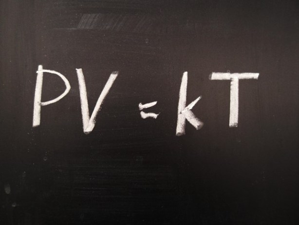
The ingenious thing is that the best part of this work is done on geometric grounds, on thinking of the spatial relationships between quantities that describe how a system moves heat around. “Spatial” may seem a strange word to describe this since we’re talking about things that don’t have any direct physical presence, like “temperature” and “entropy”. But if you draw pictures of how these quantities relate to one another, you have curves and parallelograms and figures that follow the same rules of how things fit together that you’re used to from ordinary everyday objects.

A wonderful side point is a touch of human fallibility from a great mind: in working out his relations, Maxwell misunderstood just what was meant by “entropy”, and needed correction by the at-least-as-great Josiah Willard Gibbs. Many people don’t quite know what to make of entropy even today, and Maxwell was working when the word was barely a generation away from being coined, so it’s quite reasonable he might not understand a term that was relatively new and still getting its precise definition. It’s surprising nevertheless to see.

carnotcycle

James Clerk Maxwell and the geometrical figure with which he proved his famous thermodynamic relations

Historical background

Every student of thermodynamics sooner or later encounters the Maxwell relations – an extremely useful set of statements of equality among partial derivatives, principally involving the state variables P, V, T and S. They are general thermodynamic relations valid for all systems.

The four relations originally stated by Maxwell are easily derived from the (exact) differential relations of the thermodynamic potentials:

dU = TdS – PdV   ⇒   (∂T/∂V)_S = –(∂P/∂S)_V
dH = TdS + VdP   ⇒   (∂T/∂P)_S = (∂V/∂S)_P
dG = –SdT + VdP   ⇒   –(∂S/∂P)_T = (∂V/∂T)_P
dA = –SdT – PdV   ⇒   (∂S/∂V)_T = (∂P/∂T)_V

This is how we obtain these Maxwell relations today, but it disguises the history of their discovery. The thermodynamic state functions H, G and A were yet to…

View original post 1,262 more words

The Geometry of Thermodynamics (Part 1)

I should mention that Peter Mander’s Carnot Cycle blog has a fine entry, “The Geometry of Thermodynamics (Part I)” which admittedly opens with a diagram that looks like the sort of thing you create when you want to present a horrifying science diagram. That’s a bit of flavor.

Mander writes about part of what made J Willard Gibbs probably the greatest theoretical physicist that the United States has yet produced: Gibbs put much of thermodynamics into a logically neat system, the kind we still basically use today, and all the better saw represent it and understand it as a matter of surface geometries. This is an abstract kind of surface — looking at the curve traced out by, say, mapping the energy of a gas against its volume, or its temperature versus its entropy — but if you can accept the idea that we can draw curves representing these quantities then you get to use your understanding how how solid objects (and Gibbs even got made solid objects — James Clerk Maxwell, of Maxwell’s Equations fame, even sculpted some) look and feel.

This is a reblogging of only part one, although as Mander’s on summer holiday you haven’t missed part two.

carnotcycle

Volume One of the Scientific Papers of J. Willard Gibbs, published posthumously in 1906, is devoted to Thermodynamics. Chief among its content is the hugely long and desperately difficult “On the equilibrium of heterogeneous substances (1876, 1878)”, with which Gibbs single-handedly laid the theoretical foundations of chemical thermodynamics.

In contrast to James Clerk Maxwell’s textbook Theory of Heat (1871), which uses no calculus at all and hardly any algebra, preferring geometry as the means of demonstrating relationships between quantities, Gibbs’ magnum opus is stuffed with differential equations. Turning the pages of this calculus-laden work, one could easily be drawn to the conclusion that the writer was not a visual thinker.

But in Gibbs’ case, this is far from the truth.

The first two papers on thermodynamics that Gibbs published, in 1873, were in fact visually-led. Paper I deals with indicator diagrams and their comparative properties, while Paper II

View original post 1,490 more words

The ideal gas equation

I did want to mention that the CarnotCycle big entry for the month is “The Ideal Gas Equation”. The Ideal Gas equation is one of the more famous equations that isn’t F = ma or E = mc², which I admit is’t a group of really famous equations; but, at the very least, its content is familiar enough.

If you keep a gas at constant temperature, and increase the pressure on it, its volume decreases, and vice-versa, known as Boyle’s Law. If you keep a gas at constant volume, and decrease its pressure, its temperature decreases, and vice-versa, known as Gay-Lussac’s law. Then Charles’s Law says if a gas is kept at constant pressure, and the temperature increases, then the volume increases, and vice-versa. (Each of these is probably named for the wrong person, because they always are.) The Ideal Gas equation combines all these relationships into one, neat, easily understood package.

Peter Mander describes some of the history of these concepts and equations, and how they came together, with the interesting way that they connect to the absolute temperature scale, and of absolute zero. Absolute temperatures — Kelvin — and absolute zero are familiar enough ideas these days that it’s difficult to remember they were ever new and controversial and intellectually challenging ideas to develop. I hope you enjoy.

carnotcycle

If you received formal tuition in physical chemistry at school, then it’s likely that among the first things you learned were the 17th/18th century gas laws of Mariotte and Gay-Lussac (Boyle and Charles in the English-speaking world) and the equation that expresses them: PV = kT.

It may be that the historical aspects of what is now known as the ideal (perfect) gas equation were not covered as part of your science education, in which case you may be surprised to learn that it took 174 years to advance from the pressure-volume law PV = k to the combined gas law PV = kT.

The lengthy timescale indicates that putting together closely associated observations wasn’t regarded as a must-do in this particular era of scientific enquiry. The French physicist and mining engineer Émile Clapeyron eventually created the combined gas equation, not for its own sake, but because he needed an…

View original post 1,628 more words

The Liquefaction of Gases – Part II

The CarnotCycle blog has a continuation of last month’s The Liquefaction of Gases, as you might expect, named The Liquefaction of Gases, Part II, and it’s another intriguing piece. The story here is about how the theory of cooling, and of phase changes — under what conditions gases will turn into liquids — was developed. There’s a fair bit of mathematics involved, although most of the important work is in in polynomials. If you remember in algebra (or in pre-algebra) drawing curves for functions that had x³ in them, and in finding how they sometimes had one and sometimes had three real roots, then you’re well on your way to understanding the work which earned Johannes van der Waals the 1910 Nobel Prize in Physics.

carnotcycle

Future Nobel Prize winners both. Kamerlingh Onnes and Johannes van der Waals in 1908.

On Friday 10 July 1908, at Leiden in the Netherlands, Kamerlingh Onnes succeeded in liquefying the one remaining gas previously thought to be non-condensable – helium – using a sequential Joule-Thomson cooling technique to drive the temperature down to just 4 degrees above absolute zero. The event brought to a conclusion the race to liquefy the so-called permanent gases, following the revelation that all gases have a critical temperature below which they must be cooled before liquefaction is possible.

This crucial fact was established by Dr. Thomas Andrews, professor of chemistry at Queen’s College Belfast, in his groundbreaking study of the liquefaction of carbon dioxide, “On the Continuity of the Gaseous and Liquid States of Matter”, published in the Philosophical Transactions of the Royal Society of London in 1869.

As described in Part I of…

View original post 2,047 more words

The Liquefaction of Gases – Part I

I know, or at least I’m fairly confident, there’s a couple readers here who like deeper mathematical subjects. It’s fine to come up with simulated Price is Right games or figure out what grades one needs to pass the course, but those aren’t particularly challenging subjects.

But those are hard to write, so, while I stall, let me point you to CarnotCycle, which has a nice historical article about the problem of liquefaction of gases, a problem that’s not just steeped in thermodynamics but in engineering. If you’re a little familiar with thermodynamics you likely won’t be surprised to see names like William Thomson, James Joule, or Willard Gibbs turn up. I was surprised to see in the additional reading T O’Conor Sloane show up; science fiction fans might vaguely remember that name, as he was the editor of Amazing Stories for most of the 1930s, in between Hugo Gernsback and Raymond Palmer. It’s often a surprising world.

carnotcycle

On Monday 3 December 1877, the French Academy of Sciences received a letter from Louis Cailletet, a 45 year-old physicist from Châtillon-sur-Seine. The letter stated that Cailletet had succeeded in liquefying both carbon monoxide and oxygen.

Liquefaction as such was nothing new to 19th century science, it should be said. The real news value of Cailletet’s announcement was that he had liquefied two gases previously considered ‘non condensable’.

While a number of gases such as chlorine, carbon dioxide, sulfur dioxide, hydrogen sulfide, ethylene and ammonia had been liquefied by the simultaneous application of pressure and cooling, the principal gases comprising air – nitrogen and oxygen – together with carbon monoxide, nitric oxide, hydrogen and helium, had stubbornly refused to liquefy, despite the use of pressures up to 3000 atmospheres. By the mid-1800s, the general opinion was that these gases could not be converted into liquids under any circumstances.

But in…

View original post 1,334 more words

CarnotCycle on the Gibbs-Helmholtz Equation

I’m a touch late discussing this and can only plead that it has been December after all. Over on the CarnotCycle blog — which is focused on thermodynamics in a way I rather admire — was recently a discussion of the Gibbs-Helmholtz Equation, which turns up in thermodynamics classes, and goes a bit better than the class I remember by showing a couple examples of actually using it to understand how chemistry works. Well, it’s so easy in a class like this to get busy working with symbols and forget that thermodynamics is a supremely practical science [1].

The Gibbs-Helmholtz Equation — named for Josiah Willard Gibbs and for Hermann von Helmholtz, both of whom developed it independently (Helmholtz first) — comes in a couple of different forms, which CarnotCycle describes. All these different forms are meant to describe whether a particular change in a system is likely to happen. CarnotCycle’s discussion gives a couple of examples of actually working out the numbers, including for the Haber process, which I don’t remember reading about in calculative detail before. So I wanted to recommend it as a bit of practical mathematics or physics.

[1] I think it was Stephen Brush pointed out many of the earliest papers in thermodynamics appeared in railroad industry journals, because the problems of efficiently getting power from engines, and of how materials change when they get below freezing, are critically important to turning railroads from experimental contraptions into a productive industry. The observation might not be original to him. The observation also might have been Wolfgang Schivelbusch’s instead.

From ElKement: May The Force Field Be With You

I’m derelict in mentioning this but ElKement’s blog, Theory And Practice Of Trying To Combine Just Anything, has published the second part of a non-equation-based description of quantum field theory. This one, titled “May The Force Field Be With You: Primer on Quantum Mechanics and Why We Need Quantum Field Theory”, is about introducing the idea of a field, and a bit of how they can be understood in quantum mechanics terms.

A field, in this context, means some quantity that’s got a defined value for every point in space and time that you’re studying. As ElKement notes, the temperature is probably the most familiar to people. I’d imagine that’s partly because it’s relatively easy to feel the temperature change as one goes about one’s business — after all, gravity is also a field, but almost none of us feel it appreciably change — and because weather maps make the changes of that in space and in time available in attractive pictures.

The thing the field contains can be just about anything. The temperature would be just a plain old number, or as mathematicians would have it a “scalar”. But you can also have fields that describe stuff like the pull of gravity, which is a certain amount of pull and pointing, for us, toward the center of the earth. You can also have fields that describe, for example, how quickly and in what direction the water within a river is flowing. These strengths-and-directions are called “vectors” [1], and a field of vectors offers a lot of interesting mathematics and useful physics. You can also plunge into more exotic mathematical constructs, but you don’t have to. And you don’t need to understand any of this to read ElKement’s more robust introduction to all this.

[1] The independent student newspaper for the New Jersey Institute of Technology is named The Vector, and has as motto “With Magnitude and Direction Since 1924”. I don’t know if other tech schools have newspapers which use a similar joke.

From ElKement: Space Balls, Baywatch, and the Geekiness of Classical Mechanics

Over on Elkement’s blog, Theory and Practice of Trying To Combine Just Anything, is the start of a new series about quantum field theory. Elke Stangl is trying a pretty impressive trick here in trying to describe a pretty advanced field without resorting to the piles of equations that maybe are needed to be precise, but, which also fill the page with piles of equations.

The first entry is about classical mechanics, and contrasting the familiar way that it gets introduced to people —- the whole forceequalsmasstimesacceleration bit — and an alternate description, based on what’s called the Principle of Least Action. This alternate description is as good as the familiar old Newton’s Laws in describing what’s going on, but it also makes a host of powerful new mathematical tools available. So when you get into serious physics work you tend to shift over to that model; and, if you want to start talking Modern Physics, stuff like quantum mechanics, you pretty nearly have to start with that if you want to do anything.

So, since it introduces in clear language a fascinating and important part of physics and mathematics, I’d recommend folks try reading the essay. It’s building up to an explanation of fields, as the modern physicist understands them, too, which is similarly an important topic worth being informed about.

On exact and inexact differentials

The CarnotCycle blog recently posted a nice little article titled “On Exact And Inexact Differentials” and I’m bringing it to people’s attention because its the sort of thing which would have been extremely useful to me at a time when I was reading calculus-heavy texts that just assumed you knew what exact differentials were, without being aware that you probably missed the day in intro differential equations when they were explained. (That was by far my worst performance in a class. I have no excuse.)

So this isn’t going to be the most accessible article you run across on my blog here, until I finish making the switch to a full-on advanced statistical mechanics course. But if you start getting into, particularly, thermodynamics and wonder where this particular and slightly funky string of symbols comes from, this is a nice little warmup. For extra help, CarnotCycle also explains what makes something an inexact differential.

carnotcycle

From the search term phrases that show up on this blog’s stats, CarnotCycle detects that a significant segment of visitors are studying foundation level thermodynamics at colleges and universities around the world. So what better than a post that tackles that favorite test topic – exact and inexact differentials.

When I was an undergraduate, back in the time of Noah, we were first taught the visual approach to these things. Later we dispensed with diagrams and got our answers purely through the operations of calculus, but either approach is equally instructive. CarnotCycle herewith presents them both.

View original post 835 more words

Gibbs’ Elementary Principles in Statistical Mechanics

I had another discovery from the collection of books at archive.org, now that I thought to look for it: Josiah Willard Gibbs’s Elementary Principles in Statistical Mechanics, originally published in 1902 and reprinted 1960 by Dover, which gives you a taste of Gibbs’s writings by its extended title, Developed With Especial Reference To The Rational Foundation of Thermodynamics. Gibbs was an astounding figure even in a field that seems to draw out astounding figures, and he’s a good candidate for the title of “greatest scientist to come from the United States”.

He lived in walking distance of Yale (where his father and then he taught) nearly his whole life, working nearly isolated but with an astounding talent for organizing the many complex and confused ideas in the study of thermodynamics into a neat, logical science. Some great scientists have the knack for finding important work to do; some great scientists have the knack for finding ways to express work so the masses can understand it. Gibbs … well, perhaps it’s a bit much to say the masses understand it, but the language of modern thermodynamics and of quantum mechanics is very much the language he spoke a century-plus ago.

My understanding is he published almost all his work in the journal Transactions of the Connecticut Philosophical Society, in a show of hometown pride which probably left the editors baffled but, I suppose, happy to print something this fellow was very sure about.

To give some idea why they might have found him baffling, though, consider the first paragraph of Chapter 1, which is accurate and certainly economical:

We shall use Hamilton’s form of the equations of motion for a system of n degrees of freedom, writing $q_1, \cdots q_n$ for the (generalized) coördinates, $\dot{q}_1, \cdots \dot{q}_n$ for the (generalized) velocities, and

$F_1 q_1 + F_2 q_2 + \cdots + F_n q_n$ [1]

for the moment of the forces. We shall call the quantities $F_1, \cdots F_n$ the (generalized) forces, and the quantities $p_1 \cdots p_n$ , defined by the equations

$p_1 = \frac{d\epsilon_p}{d\dot{q}_1}, p_2 = \frac{d\epsilon_p}{d\dot{q}_2}, etc.,$ [2]

where $\epsilon_p$ denotes the kinetic energy of the system, the (generalized) momenta. The kinetic energy is here regarded as a function of the velocities and coördinates. We shall usually regard it as a function of the momenta and coördinates, and on this account we denote it by $\epsilon_p$ . This will not prevent us from occasionally using formulas like [2], where it is sufficiently evident the kinetic energy is regarded as function of the $\dot{q}$ ‘s and $q$ ‘s. But in expressions like $d\epsilon_p/dq_1$ , where the denominator does not determine the question, the kinetic energy is always to be treated in the differentiation as function of the p’s and q’s.

(There’s also a footnote I skipped because I don’t know an elegant way to include it in WordPress.) Your friend the physics major did not understand that on first read any more than you did, although she probably got it after going back and reading it a touch more slowly. And his writing is just like that: 240 pages and I’m not sure I could say any of them could be appreciably tightened.

Also, I note I finally reached 9,000 page views! Thank you; I couldn’t have done it without at least twenty of you, since I’m pretty sure I’ve obsessively clicked on my own pages at minimum 8,979 times.

J Willard Gibbs.

Kindly share this:

Buffon’s Needle.

Kindly share this:

Kindly share this:

Kindly share this:

Kindly share this:

Sorites Paradox.

Kindly share this:

Nearest Neighbor Model.

Kindly share this:

Infinite Monkey Theorem.

Kindly share this:

Distribution (probability).

Kindly share this:

Kindly share this:

Kindly share this:

Kindly share this:

Kindly share this:

Ergodic.

Kindly share this:

Distribution (statistics)

Kindly share this:

Kindly share this:

Kindly share this:

Kindly share this:

Kindly share this:

Kindly share this:

Kindly share this:

Kindly share this:

Kindly share this:

Kindly share this:

Kindly share this:

Kindly share this:

Kindly share this:

Kindly share this:

Kindly share this:

Kindly share this:

Kindly share this:

Kindly share this:

Kindly share this: